How to compute the Solvent Accessible Surface Areas (SASA) with GROMACS

The Solvent Accessible Surface Area (SASA) of proteins is a decisive factor in the study of protein folding and stability.

For this reason, in GROMACS you will find a dedicated tool to compute this essential structural feature. In this article, I will give you a general idea of what is the SASA and how you can compute it using the built-in GROMACS module gmx sasa. Finally, you will also learn how to plot the results of this analysis.

Solvent Accessible Surface Area (SASA)

As the name suggests, the Solvent Accessible Surface Area (SASA) is a measure of the surface area of a biomolecule (e.g., protein) or other molecular structures that is accessible by the solvent molecules. It is defined as the extent to which atoms on the surface of a protein can form contact with the solvent, and it is generally measured in squared nanometers (nm$^2$).

SASA is a quantity of particular interest in protein folding and functional studies. It plays an important role to understand the structure-function relationship of proteins and their residues and is commonly used in computational studies of proteins. For instance, the burial of hydrophobic residues can be a key factor in protein folding, and the exposure of these residues to the solvent and the hydrophobic core is directly related to the stability of the protein.

The SASA is calculated by considering the surface of the molecule as a series of points, and then using a probe, typically a sphere, to trace out the accessible surface area. Different algorithms and computational tools are nowadays available to estimate the SASA. One of the simplest and oldest ones is a numerical method named Shrake–Rupley algorithm.

This method draws 92 points equidistant from each atom of the molecule and uses the number of these points that are solvent-accessible to determine the surface area. The number of exposed atoms determines the proportion of the total surface area that is accessible to the solvent.

The algorithm implemented in GROMACS is an algorithmic variant of this approach showing improvements to speed up the calculations. It is named The Double Cubic Lattice Method (DCLM).

The gmx sasa command

Below you can find a couple of examples of how you can use the gmx sasa implementation of GROMACS to compute:

• The SASA value for a static protein structure in the pdb or gro format.
• The evolution of the SASA during a simulation run.

How to compute SASA for a protein structure

First of all, let’s see how you can use the gmx sasa module to compute the SASA for your protein. For this analysis, we just need the structure of your protein in the gro or pbd format (protein.gro, protein.pdb).

1

gmx sasa -f protein.pdb -s protein.pdb -o sasa.xvg 

You will be prompted to specify a group for the surface calculation which should consist of all non-solvent atoms. If you want to compute the SASA for your protein you need to select Group 1 "Protein". You can also directly specify it from the command line by adding -surface Protein.

You will find the SASA value for your protein in the output file in the xvg format (sasa.xvg). You can open it with your favorite text editor.

How to compute the SASA along a simulation

In most cases, you will be interested in the evolution of the SASA along the course of the simulation. You can do it with the following command:

1

gmx sasa -f simulation.xtc -s system.tpr -o sasa.xvg (-tu ns)

As in the previous case, you will be asked to specify a group for the surface calculation which should consist of all non-solvent atoms. In case you want to compute the SASA for your protein you need to select Group 1 "Protein". You can also directly specify it from the command line by adding -surface Protein.

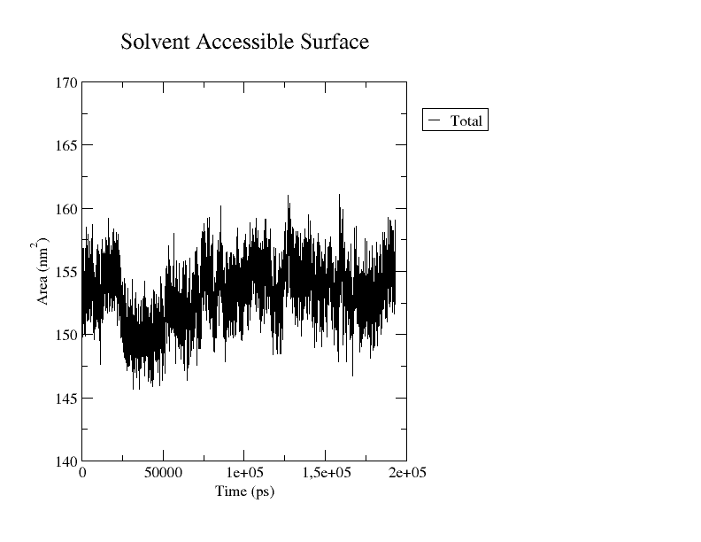
The output file is an xvg file that you can plot as you wish. Here I showed you how to plot an xvg file with Grace or Python.

If you choose to use Xmgrace, you’ll obtain a plot similar to the one reported below, depicting the surface area (in nm²) as a function of time (in ps).

1

xmgrace sasa.xvg