How to extract and plot thermodynamic properties from a GROMACS simulation

GROMACS is one of the most widely packages to perform Molecular Dynamics (MD) simulations.

In previous articles, I showed you the basic commands required to carry out the different steps of an MD simulation.

However, running a simulation should just be the tip of the iceberg. Hopefully, one would also like to extract some information from the run. Right?

One of the main strengths of GROMACS is that it also comes with a broad range of tools to perform analysis on your system.

In this article, I will show you how to extract the thermodynamic properties from your simulation using the gmx energy command.

The gmx energy command

During a simulation, it is important to monitor a series of different thermodynamic properties to always make sure that everything is proceeding according to our plans. To this aim, we use the gmx energy command.

This command simply takes an edr file as input and returns an output file in the xvg format which can be used to plot our data. Later I will show you how to plot them using Python or Xmgrace.

The syntax is quite easy:

1

gmx energy -f simulation.edr -o property.xvg 

Once you launched the command you will be asked to choose which property you want to obtain. Something like this code block below.

 1
 2
 3
 4
 5
 6
 7
 8
 9
10
11
12
13
14
15
16
17
18
19
20
21

Command line:
  gmx_mpi energy -f system.edr -o property.xvg

Opened system.edr as single precision energy file

Select the terms you want from the following list by
selecting either (part of) the name or the number or a combination.
End your selection with an empty line or a zero.
-------------------------------------------------------------------
  1  U-B              2  Proper-Dih.      3  Improper-Dih.    4  Improper-Dih.
  5  CMAP-Dih.        6  LJ-14            7  Coulomb-14       8  LJ-(SR)
  9  Disper.-corr.   10  Coulomb-(SR)    11  Coul.-recip.    12  Position-Rest.
 13  Dih.-Rest.      14  Potential       15  Kinetic-En.     16  Total-Energy
 17  Conserved-En.   18  Temperature     19  Pres.-DC        20  Pressure
 21  Constr.-rmsd    22  Vir-XX          23  Vir-XY          24  Vir-XZ
 25  Vir-YX          26  Vir-YY          27  Vir-YZ          28  Vir-ZX
 29  Vir-ZY          30  Vir-ZZ          31  Pres-XX         32  Pres-XY
 33  Pres-XZ         34  Pres-YX         35  Pres-YY         36  Pres-YZ
 37  Pres-ZX         38  Pres-ZY         39  Pres-ZZ         40  #Surf*SurfTen
 41  T-Protein_membrane                  42  T-solvent
 43  Lamb-Protein_membrane               44  Lamb-solvent

From here, you can select the property you want to extract by simply typing the corresponding number followed by a 0.

To obtain an xvg file for the temperature you can type:

1

18 0 

Plotting data in the xvg format

Now that we have our xvg file we can create a plot to observe how the selected property evolved along the simulation.

This is particularly important during the equilibration phase of our experiment. During this step, we have to monitor different properties of our system to make sure that everything is correct.

Here I will show you two different ways to plot an xvg file format.

Xmgrace

The first tool we are going to use to plot the data in the xvg file is Grace.

This plotting program is perfectly able to handle a file in the xvg format. It is quite fast and intuitive and it is particularly useful when you just need a quick plot.

1

brew install grace

1

sudo apt-get install grace

Let’s assume that you generated a volume.xvg file that you want to investigate, and that you have Grace installed. You can easily plot the file with the following command:

1

xmgrace volume.xvg

As a result you will get a plot like the one displayed below.

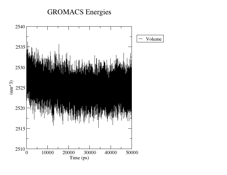
Volume variation as a function of time ($ps$) plotted with Grace

To save the image in the .png format you can enter the following:

1

xmgrace -nxy volume.xvg -hdevice PNG -hardcopy -printfile volume.png

Python

if you are more of a Python type don’t worry. You can still plot an .xvg file using numpy, and matplotlib.

1
2
3
4
5
6
7
8
9

import matplotlib.pyplot as plt
import numpy as np

x,y = np.loadtxt("volume.xvg",comments=["@", "#"],unpack=True)
plt.plot(x,y)
plt.xlabel("time (ps)")
plt.ylabel("volume (nm^3)")
plt.savefig("volume.png", format="png", dpi=300)
plt.show()

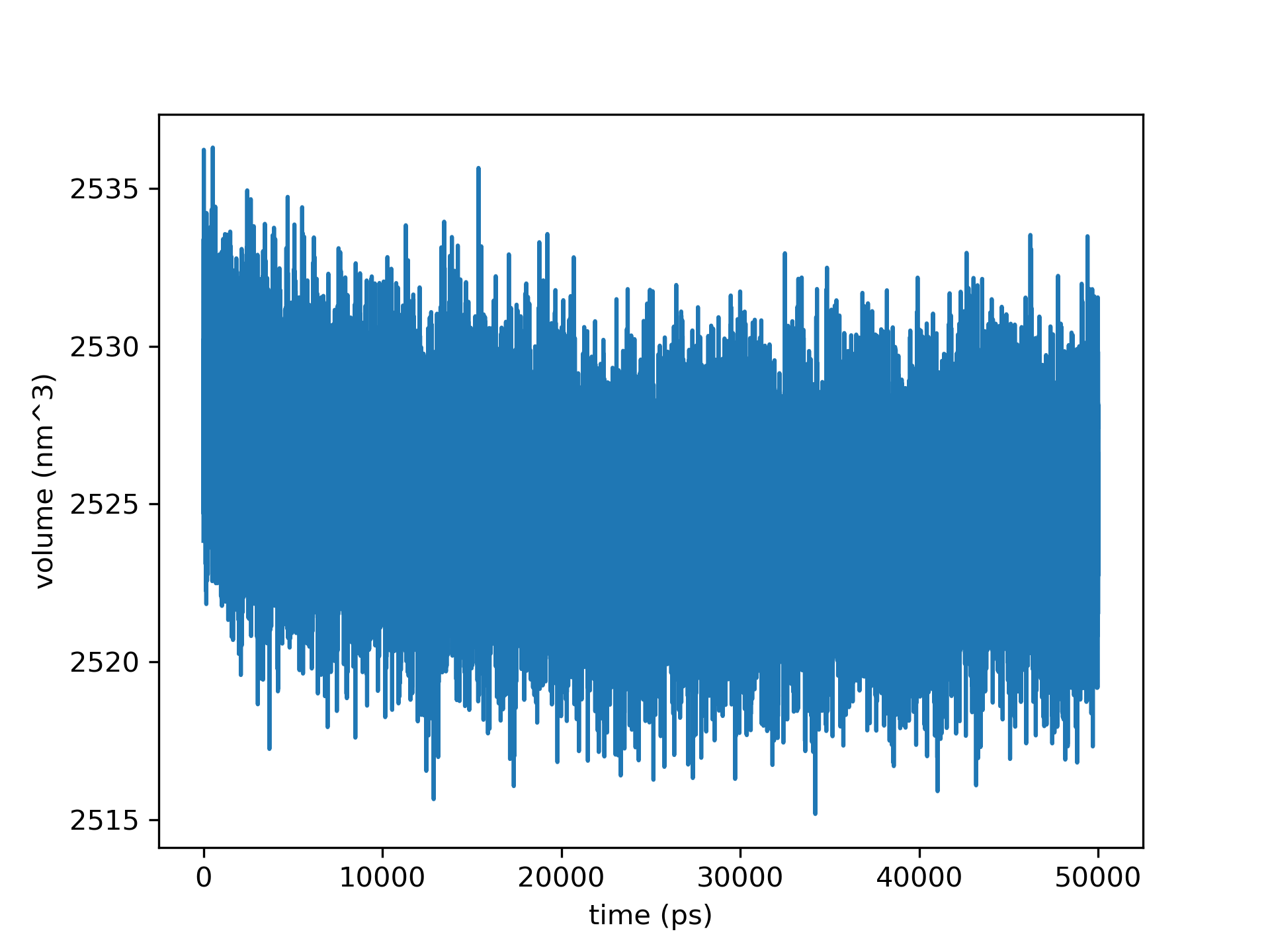
Volume variation as a function of time ($ps$) plotted with Python

Example

Here I will show you a realistic example of how to retrieve information using the gmx energy command, and the Grace plotting tool.

Let’s say that you have just finished your equilibration step in the NPT ensemble, and you want to check that everything looks right.

The first step is to take the generated edr file (that we will call npt.edr) and extract relevant properties. A common practice is to consider at least six quantities:

• Temperature
• Volume
• Pressure
• Kinetic energy
• Potential energy
• Total energy

So for each one of them you need to generate the corresponding .xvg file. You can do this by typing the following six commands.

1
2
3
4
5
6

gmx_mpi energy -f npt.edr -o temperature.xvg
gmx_mpi energy -f npt.edr -o volume.xvg
gmx_mpi energy -f npt.edr -o pressure.xvg
gmx_mpi energy -f npt.edr -o kinetic.xvg
gmx_mpi energy -f npt.edr -o potential.xvg
gmx_mpi energy -f npt.edr -o total.xvg

For each line, you will be asked to select the property followed by a 0. In the end, you will have six xvg files.

You can generate a png image with the corresponding plot for each of the files with a simple bash script.

Create a text file (images.sh) and paste the following code.

1
2
3
4
5
6

  #!/bin/bash
  
  for i in *xvg
  do
  xmgrace -nxy $i -hdevice PNG -hardcopy -printfile ${i:0:-4}.png
  done

Run it with bash

1

bash images.sh

Now you have your images containing the plots to monitor the quantities of your simulation.

Another common property to monitor during an equilibration step is a structural feature named Root Mean Square Deviation (RMSD). Here I show you how to compute the RMSD using GROMACS.

How to merge two edr energy files

In some cases, you may happen to run a simulation for some time without getting relevant results. In such circumstances you can decide to extend the simulation for some additional time.

When extending the simulation you can result in two different energy edr files.

We can use the gmx eneconv command to merge them. The resulting edr file can be used to extract the properties from the entire simulation.

1

gmx eneconv -f simulation_1.edr simulation_2.edr -o merged.edr (-settime)