What is the RMSD and how to compute it with GROMACS

GROMACS is a powerful open source molecular simulation packages allowing us to run a Molecular Dynamics (MD) simulation, and analyze the resulting trajectories.

Among many tools, at our disposal, we have a specific command to compute the RMSD.

Here I explain to you why the RMSD is an important structural feature in molecular modeling, and how to compute it with GROMACS.

RMSD in Molecular Dynamics

The Root Mean Square Deviation (RMSD) measures how much a certain molecular structure deviates from a reference geometry.

This feature plays a key role in the field of molecular modeling, and you will find it referenced in various papers.

But why is it so important?

In Molecular Dynamics (MD), we are interested in how our system evolves over time as compared to its starting structure. For this reason, plotting the RMSD as a function of time can help us in two ways:

• First of all, it is useful to identify parts of the simulation where we have important changes in the structure. For example, if a protein over the course of the simulation has some large conformational changes we should notice a spike in the RMSD vs. time plot.

• As a second point, The RMSD is commonly used as an indicator of convergence of the structure towards an equilibrium state. A flattening of the RMSD curve can indicate that the protein has equilibrated and that we can proceed with the next step.

Therefore, the RMSD has a critical role in the different steps of an MD simulation (i.e., equilibration and production runs).

The equation for RMSD

Let’s discuss the formula needed to compute this fundamental structural feature.

For a general molecular structure with $N$ atoms, we can compute the RMSD between a certain conformation ($r$) and a reference structure ($r^{ref}$) via the following equation:

$$ RMSD = \sqrt{\frac{1}{N}\displaystyle\sum_{i=1}^N(r_i - r_i^{ref})^2} $$

where $r_i^{ref}$ represents the set of coordinates of the $i$-th atom in the reference structure, while $r_i$ is the set of coordinates of the same atom but belonging to the structure that is going to be compared to the reference.

$$ r_i = x_i + y_i + z_i $$ $$ r_i^{ref} = x_i^{ref} + y_i^{ref} + z_i^{ref} $$

In summary, the RMSD is the square root of the average of the squared distances between atoms.

During a simulation, we actually compute the RMSD as a function of time $t$.

At each time step, we compute the RMSD between the coordinates at that specific time step $r(t)$, and the reference.

$$ RMSD(t) = \sqrt{\frac{1}{N}\displaystyle\sum_{i=1}^N(r_i(t) - r_i^{ref})^2} $$

In this way, we can see how the system deviates from the reference structure during our MD simulation.

The gmx rms command

In GROMACS we compute the RMSD via the gmx rms command.

The workflow for this command is quite intuitive. You only need two things:

• A reference geometry in the tpr or gro format
• A trajectory file that is going to be compared to the reference (xtc file)

GROMACS will output a file in the xvg format that you can plot using Grace or Python as I showed in this article .

Here I am going to show you a few examples of how you can play with the gmx rms command to compute the RMSD of your system.

RMSD of a trajectory

First of all, we are going to consider the most basic example.

How can we use the gmx rms command to measure the RMSD fluctuation of the system along the simulation?

In other words, we want to observe how much the structure of the system deviates from the starting one.

In GROMACS this is accomplished by comparing each frame in the trajectory file with the reference structure.

To this aim, you can type the following:

1

gmx rms -f simulation.xtc -s reference.tpr -o rmsd.xvg (-tu ns)

At this stage, you will be prompted to select two groups.

1. The group for least square fits: structure under -f flag

 1
 2
 3
 4
 5
 6
 7
 8
 9
10
11
12
13
14

Select group for least squares fit
Group     0 (         System) has 235551 elements
Group     1 (        Protein) has  4386 elements
Group     2 (      Protein-H) has  2147 elements
Group     3 (        C-alpha) has   268 elements
Group     4 (       Backbone) has   804 elements
Group     5 (      MainChain) has  1071 elements
Group     6 (   MainChain+Cb) has  1334 elements
Group     7 (    MainChain+H) has  1330 elements
Group     8 (      SideChain) has  3056 elements
Group     9 (    SideChain-H) has  1076 elements
Group    10 (    Prot-Masses) has  4386 elements
Group    11 (    non-Protein) has 231165 elements
Group    12 (          Other) has 231165 elements

2. The group for RMSD calculation: structure under -s flag

 1
 2
 3
 4
 5
 6
 7
 8
 9
10
11
12
13
14

Select group for RMSD calculation
Group     0 (         System) has 235551 elements
Group     1 (        Protein) has  4386 elements
Group     2 (      Protein-H) has  2147 elements
Group     3 (        C-alpha) has   268 elements
Group     4 (       Backbone) has   804 elements
Group     5 (      MainChain) has  1071 elements
Group     6 (   MainChain+Cb) has  1334 elements
Group     7 (    MainChain+H) has  1330 elements
Group     8 (      SideChain) has  3056 elements
Group     9 (    SideChain-H) has  1076 elements
Group    10 (    Prot-Masses) has  4386 elements
Group    11 (    non-Protein) has 231165 elements
Group    12 (          Other) has 231165 elements

For protein simulations, it is a common practice to compute the “backbone to backbone” RMSD value (Select group “4” for both).

You can automate the selection with this command:

1

printf "4 4" | gmx_mpi rms -f md.xtc -s md.tpr -o rmsd.xvg

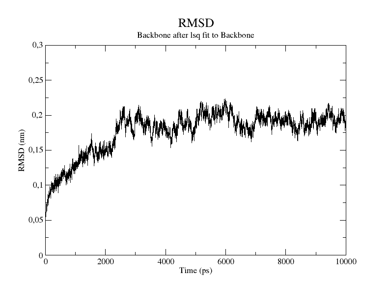
The resulting rmsd.xvg file can be plotted with Grace.

1

xmgrace rmsd.xvg

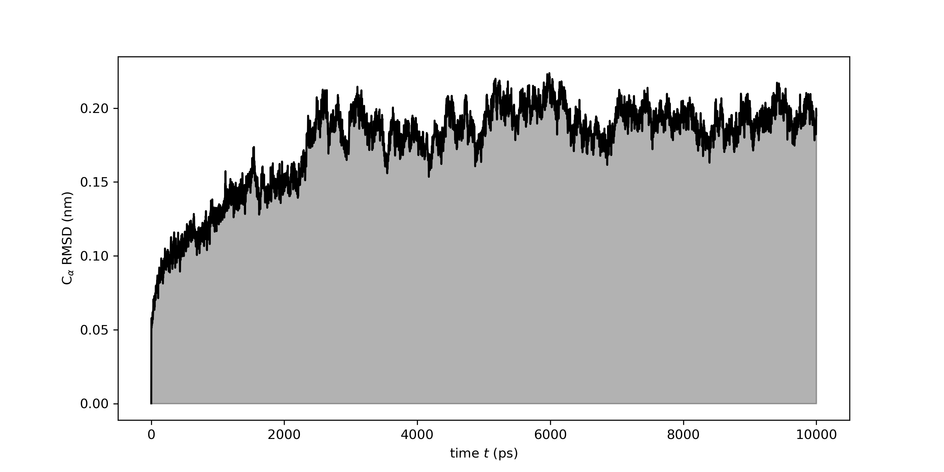
Or with Python using the Numpy and Matplotlib libraries.

 1
 2
 3
 4
 5
 6
 7
 8
 9
10
11
12
13
14
15
16
17
18
19
20
21
22
23
24
25
26

# Importing the necessary libraries for plotting
import matplotlib.pyplot as plt
import numpy as np

# Loading data from the rmsd.xvg file, ignoring lines starting with "@" or "#"
t,rmsd = np.loadtxt("rmsd.xvg", comments=["@", "#"], unpack=True)

# Creating a figure and axis objects for the plot
fig = plt.figure(figsize=(10,5))
ax = fig.add_subplot(111)

# Filling the area between the x-values (res) and y-values (rmsf) with a semi-transparent black color
ax.fill_between(t,rmsd, color="black", linestyle="-", alpha=0.3)

# Plotting the line representing the RMSF values
ax.plot(t,rmsd, color="black", linestyle="-")

# Setting labels for the x-axis (time in ps) and y-axis (RMSD value)
ax.set_xlabel("time $t$ (ps)")
ax.set_ylabel(r"C$_\alpha$ RMSD (nm)")

# Saving the plot as a PNG image with higher resolution (300 dpi)
plt.savefig("rmsd.png", format="png", dpi=300)

# Displaying the plot
plt.show()

RMSD for a specific part of the system

If you want to analyze a specific part of your system that is not within the default GROMACS groups you can create an index with the gmx make_ndx command.

Subsequently, you can pass the special index that you created to the gmx rms command.

1

gmx rms -f simulation.xtc -s reference.tpr -o rmsd_index.xvg -n index.ndx

RMSD for a specific time frame

You can compute the RMSD for a specific time frame of your trajectory by using the -b and -e flags.

For instance, if you are only interested in measuring the RMSD between 1000 ps and 2000 ps of your trajectory you can use the following command.

1

gmx rms -f simulation.xtc -s reference.tpr -o rmsd_time.xvg -b 1000 -e 2000

By selecting the same value for the -b and -e flags you will get the RMSD value between the reference and the frame corresponding to the time you selected.