Setting up a Molecular Dynamics simulation
Setting up a realistic simulation of a given molecular system involves different steps some of which depend on its complexity, and on the conditions we choose for our experiment.
In this article, I try to explain to you which are the typical steps to perform in Molecular Dynamics (MD). However, always keep in mind that an MD simulation protocol is highly system-dependent. Therefore, each system needs to be analyzed differently.
Pre-simulation decisions
Before starting a simulation procedure we have at least three fundamental decisions to make.
- Select the level of theory to use for our protocol.
- Decide which software we want to use for our experiment.
- Choose which is the most appropriate force field for our system.
1. Level of theory
The first necessary step is to decide which energy model we want to use to describe atomic interactions. This mostly depends on the size of the system we are studying, and on the entity of the process, we are interested in.
Modeling large molecular structures often requires low levels of theory that are less computationally expensive (i.e., Molecular Mechanics, coarse-grained). On the contrary, we may choose quantum mechanical-based methods, also known as ab-initio, to model smaller systems.
In recent years, hybrid methods such as QM/MM and MM/CG techniques combining the previous methods are rapidly establishing themselves as promising tools to perform simulations.
2. Software
The selection of the technique to use is just the tip of the iceberg. As a second point, we need to select the molecular simulation program we want to use.
Different valid alternatives are nowadays available. The most famous are:
Feel free to explore, and choose the one you prefer. Keep in mind that for some of them you will need a license.
3. Force Field
As the last step, we need to select the force field that is more suited for our specific case. Mainly depending on the type of system, we are going to consider.
Search in the literature which type of force field is more common in your field. Also, remember to check the compatibility between the force field and the molecular simulation package.
Setup the simulation
Finally, we are ready to start the experiment.
A Molecular Dynamics simulation can be divided into mainly four steps:
- System preparation
- Minimization
- Equilibration
- Production
Let us consider each of these steps more in-depth.
Putting this into practice? This article maps out the stages; my GROMACS protein-in-water guide turns them into a concrete, runnable project, from PDB file to analysed trajectory, with every MDP file, command and script included. Get the guide →
System preparation
The first step of an MD simulation consists of preparing the system we need to analyze. In other words, before proceeding with the experiment it is necessary to provide an initial configuration of the system. This choice needs to be exercised with great care as it can determine the success or failure of a simulation. Indeed, starting from an imprecise structure may lead to enormous errors in the subsequent steps.
The structure can be obtained from experimental or computational techniques, or by combining the two approaches. Ideally, we would like to have a starting structure that highly resembles the equilibrium configurations. By doing so we would simply be able to reduce the time needed to stabilize the system during the equilibration step.
Once we retrieved our initial configuration we need a few additional steps to properly refine our molecular system. This editing process involves multiple steps:
- Set a simulation box: first of all, we need to set a virtual box containing our molecule. Then we implement pbc to simulate its bulk properties. Practically, we generate replicas of our box in all directions allowing us to simulate a large system starting from a small box.
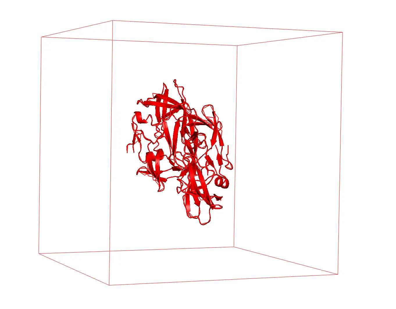
Figure 1 Protein inside a cubic box. (HIV-1 protease PDB ID: 1A8K)
- Solvation: in the second step we need to solvate our system, using $H_2O$ for instance.
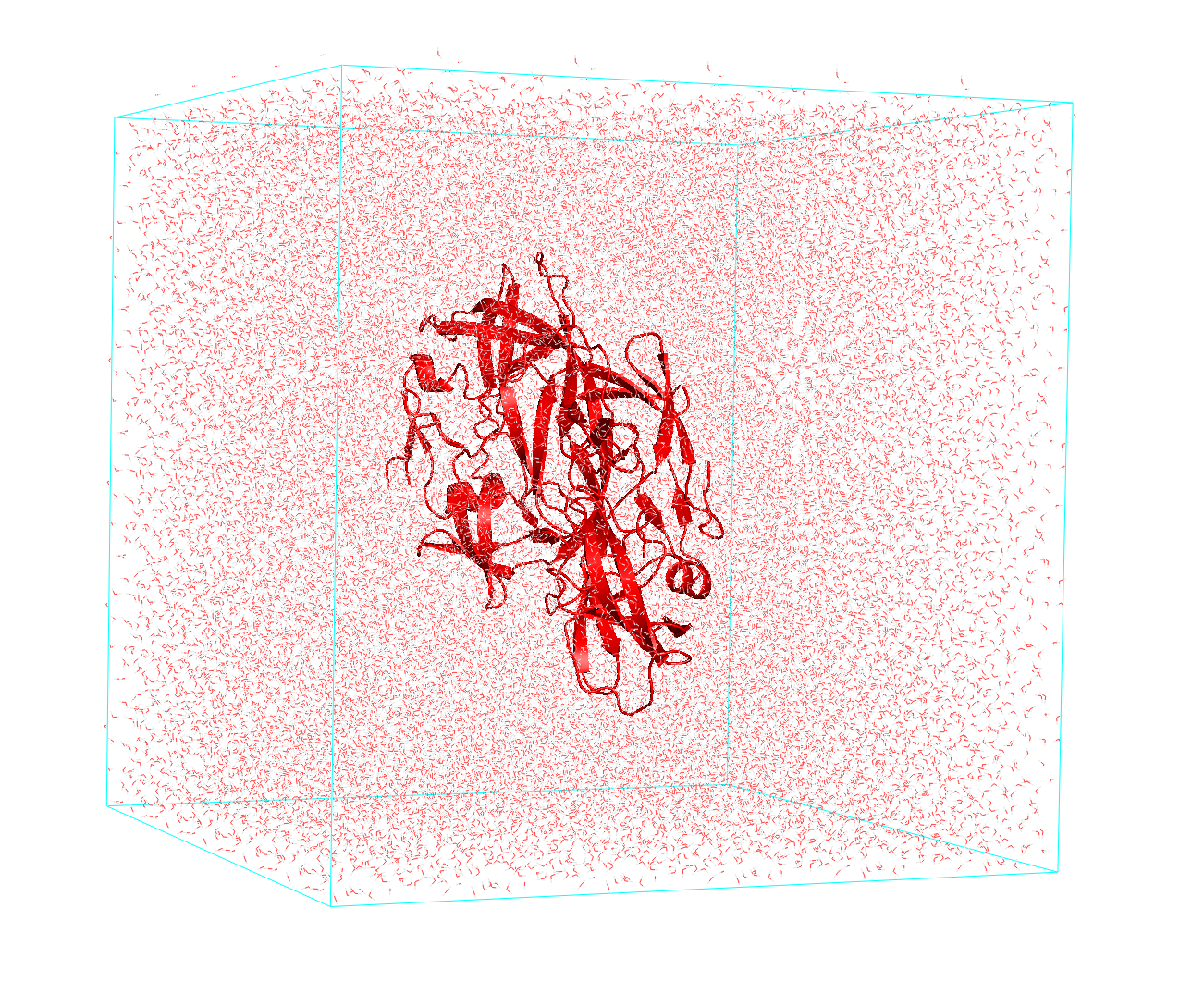
Figure 2 Protein embedded in water.
- Neutralization: In the final step we need to make the charge null. We can balance the charge by adding the appropriate counterions ($Na^+$, $Cl^-$) which will take the place of solvent molecules.
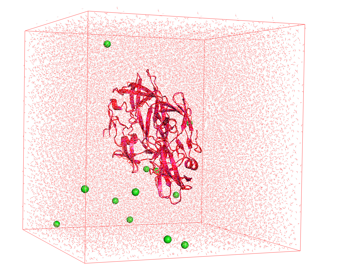
Figure 3 The charge of the protein is balanced with $Cl^-$ ions (green spheres)
Minimization
In this step what we need to do is minimize the energy of our system through the steepest descent method. The aim is to minimize energy by adjusting the coordinates of the protein to avoid clashes between atoms, which would artificially raise the energy of the system. Every minimization step will correspond to a different set of coordinates representing a lower potential energy state of our protein.
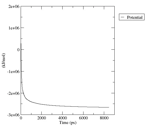
Figure 4 Potential energy decreasing as a function of time ($ps=10^{-12}s$)
The minimization process is just one step of the optimization process and it provides us with a potential energy minimum without taking into account the kinetic energy. Therefore we need further analysis to optimize the system and run the MD simulation.
At this stage, we have the coordinates of our system. However, before proceeding further with the experiment we must also assign the initial velocities of the atoms. Otherwise, we will not be able to retrieve the motion of the system. If this is not clear to you check out this article on how it is possible to acquire the motion of a system in Molecular Dynamics.
The initial velocities ($v_i$) are selected from a Maxwell-Boltzmann distribution at the temperature of interest.
$$ P(v_i) = \sqrt{\frac{m_i}{2\pi k_b T}} \exp \left(-\frac{m_i v_i^2}{2k_B T}\right) $$
where $P(v_i)$ is the probability that an atom $i$ with mass $m_i$ has velocity $v_i$ at temperature $T$. The velocities need to be adjusted so that the total momentum of the system is null, preventing the simulation box from drifting.
Equilibration
Once the initial conditions of our experiment have been clarified we can proceed to the first part of an MD experiment, namely the equilibration phase. In this stage, starting from the initial configuration, we bring the system to equilibrium, meaning that various parameters need to be monitored until they reach stable values. The parameters we need to consider largely depend on the type of thermodynamical ensemble we choose for our simulation.
For stability purposes, it is generally desirable to at least perform an equilibration run at constant temperature, and volume before moving to the production phase. Therefore, an NVT equilibration run is typically the first step. So we perform a short simulation at constant volume (V) and temperature (T) while the pressure (P) will adjust.
The second equilibration step generally consists of a simulation at constant pressure (NPT ensemble). This means that we keep P and T constant while the volume will equilibrate. In this way, we make sure that we have the correct density for the production run.
However, there are many other parameters we may consider such as temperature, pressure, volume, kinetic, potential, and total energy. These quantities should be allowed to fluctuate during the course of our experiment, but they should not deviate excessively from the starting structure.
The main quantity that we need to check to see if the system has finally reached equilibrium is the Root Mean Square Deviation (RMSD).
By plotting the RMSD measures as a function of time we can see how much the structure of the system is deviating from its original configuration. Once the RMSD fluctuates around constant values, and it does not change in time we can consider it to be at the equilibrium geometry, so we can move to the next phase. The RMSD curve for an equilibrated system should resemble Figure 5.
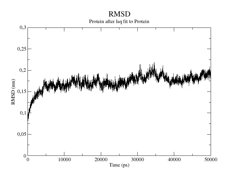
Figure 5 Change in RMSD value as a function of time ($ps=10^{-12}s$).
As you can see the RMSD immediately increases signaling that the protein undergoes a large deviation from the starting structure at the beginning of the simulation. After 5000 $ps$ the protein reaches its stable configuration, and the RMSD remains more or less constant.
The system is ready for the production run.
Production
The final step of an MD simulation is the production phase. This process still consists of a simulation carried within a certain ensemble, such as NPT or NVT. Always keep in mind that reactions in the lab are generally carried at constant pressure, so the NPT is the ensemble that mostly resembles a real experiment, and is usually preferred.
The main difference with the equilibration step is that, in this phase, we are not interested in equilibrating the system, but rather in collecting data regarding the molecule of interest. The result of the production run is therefore the ultimate goal of an MD experiment. During this final stage, we produce a trajectory describing the motion of the molecule, which can be:
- Visualized using molecular visualization software to see how its structure changes
- Used to study the behavior and the properties of our molecule.