Molecular Dynamics: Periodic Boundary Conditions (PBC)

Molecular Dynamics (MD) is an extremely powerful computational tool that allows simulating the motion of a molecule. We already underlined the mathematics required for this technique, which involves solving the equations of motion for the atoms in our system. We also highlighted the various steps needed to set up a MD experiment.

In this article, I will show you the reasons behind the implementation of the so-called Periodic Boundary Conditions, a key topic in the computational simulation of molecular structures.

Simulation of bulk systems

In recent years, great efforts have been made to increase the available computational resources. Despite that, we are still far from being able to simulate a real macroscopic system, which can be considered as composed of roughly $10^{23}$ atoms.

Nowadays, a typical MD simulation comprises a number of atoms ranging from thousands to millions. In such conditions, a large number of atoms would belong to the boundaries of the simulation box. This situation is not appropriate to derive the bulk properties of the system as the majority of atoms are within the influence of the walls.

When considering an MD simulation it is, therefore, crucial to mention how we deal with this problem, generally referred to as boundary effect.

To simulate bulk systems we need to implement Periodic boundary conditions. The essential idea behind this method is that we can simulate an infinite system by simply considering multiple repetitions of our initial finite system.

This technique exploits a concept of statistical mechanics named ergodicity which states that:

So instead of considering a large number of molecules, we can simply study a single molecule for a long enough time scale.

A two-dimensional case study

Let’s explain from a practical point of view how the periodic boundary condition is achieved, and highlight the main advantages of this technique. For simplicity purposes, we will consider two-dimensional examples but the same applies to a real simulation in three dimensions.

In other articles we saw that the first step of an MD experiment consists of constructing a virtual simulation box containing the system.

Figure 1 Box containing the particles we want to simulate (red)

Then, the box is exactly replicated in every direction in space forming an infinite lattice.

Figure 2 The central box is replicated in every direction. The replica particles are represented in blue.

As the molecules in the central box move, the ones in the replicated boxes move in the same way. During the simulation, if a molecule goes out of the box there is another one that enters from the opposite side due to the replicas so that the number of atoms is conserved. By doing so, periodic boundary conditions enable particles to experience forces as if they were in a bulk solution.

Figure 3 As soon as a red particle goes out of the box its replica replaces it.

One may think that replicating the system a large amount of times simply increases the size of the problem. In principle, we still need to find the positions of atoms in the replicas and simulate their motions. We can prove with an example that this is not the case.

Imagine we have a two-dimensional simulation box containing our molecule $A$. The box will have size $L$ in each of the two components of space $(L_x, L_y)$, and it will be replicated in every direction.

$$ L = (L_x, L_y) $$

Knowing the coordinates of the molecule $A=(x, y)$ we also know that the copied molecules in the neighboring replicated cells are simply shifted by the size of the box $(x \pm L_x, y \pm L_y)$. Correspondingly, if we replicate the cell for $n$ times the copies of each molecule will be at coordinates $(x \pm n_xL_x, y \pm n_y L_y)$, with $(n_x, n_y)$ ranging from $-\infty$ to $+\infty$.

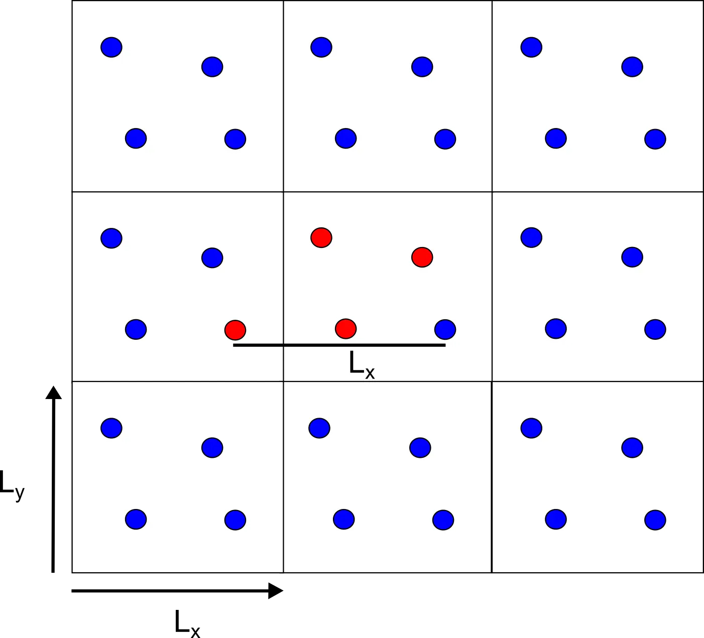
Figure 4 The replicas are exactly separated by the size of the box.

At this stage, it should be clear that the main advantage of periodic boundary conditions is that to compute the distances between different particles the only information required is the size of the box.

If that is the case, there is no need to integrate the molecules in the replicas, because at each time their position can be retrieved by simply considering the reference system. Consequently, we can decrease the computational cost of the experiment by exploiting the periodicity.

Minimum image convention and cut-off radius

In other sections we highlighted the importance of non-bonding terms produced by electrostatic and Van der Waals (VdW) interactions. The number of these terms increases with the square of the number of atoms $N^2$, and they represent the most time-consuming part of the construction of a molecular model.

Until now we did not specify how we deal with the number of interactions we have to compute in our periodic system.

Let’s analyze this topic more in-depth.

The implementation of periodic boundary conditions may lead to some problems. For instance, we may generate a situation in which a certain atom interacts with itself, or with several copies of another atom.

The minimum image convention is needed to avoid these circumstances.

This method makes sure that each atom only experiences at most just one image of every other atom in the system. In other words, the interactions are only computed with the closes image of the same atom in different replicas.

Another common practice to deal with non bonding interactions is to insert a cut-off radius ($r_{cut-off}$) beyond which the interaction will not be evaluated. This is required to speed up the calculations.

But also to make sure that we fulfil the minimum image convention. The cut-off radius needs to be chosen so that a particle does not see its own replica, or the same particle twice. For this condition to be ensured the size of the radius should not exceed half the size of the box when considering a cubic box.

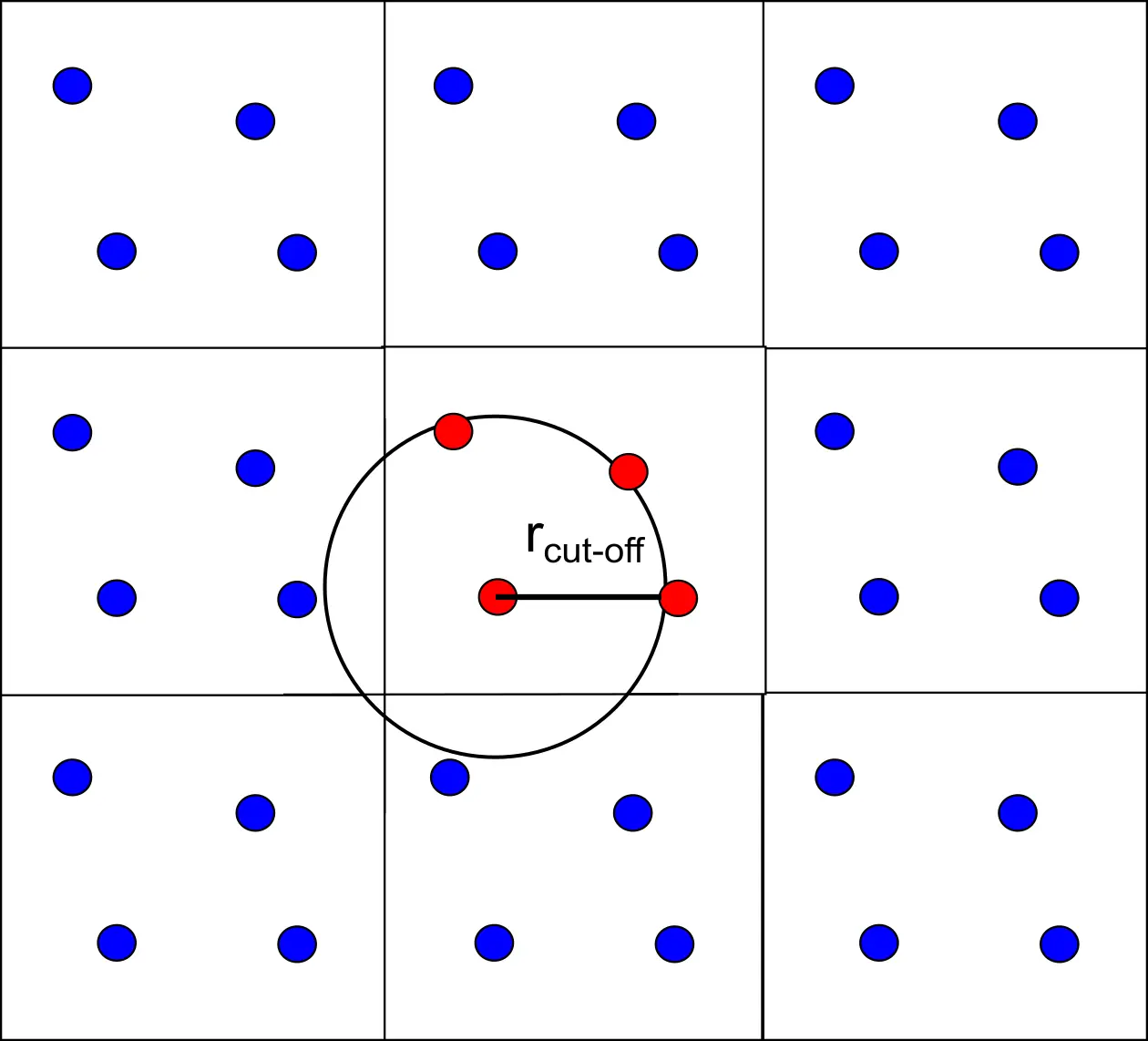
Figure 5 The interactions exceeding the cut-off value are set to zero.

Potential truncation

Due to the cut-off, we have a truncation of the potential energy of the system, meaning that the contributions above a given radius are not computed. This is not a problem for bonding terms which are short-range interactions, and are not relevant at distances larger than $r_{cut}$.

It is however inaccurate to describe the non-bonding interactions which are long-range forces, and still provide significant contributions even at larger distances.

Let’s plot the two functions for the Coulombic and Van der Waals (Lennard-Jones) interactions and see what happens when the distance increases. The Python code to do that is reported below.

 1
 2
 3
 4
 5
 6
 7
 8
 9
10
11
12
13
14
15
16
17
18
19
20
21
22
23
24
25
26
27
28
29
30
31
32
33
34
35
36
37

import numpy as np 
import seaborn as sns 
import matplotlib.pyplot as plt

sns.set_style("darkgrid")  # Change the style of the plot  

# Define the distance range and the cutoff
r = np.linspace(0, 3, 100) 
cutoff_r = 2  

# Lennard-Jones potential 
sigma = 1.0 
epsilon = 1.0 
vlj = 4*epsilon*((sigma/r)**12 - (sigma/r)**6)  

# Coulombic potential 
q1 = 1.0
q2 = -1.0
k = 1.0
vcoul = k*q1*q2/r  

# Create a plot 

fig, ax = plt.subplots(figsize=(8,6)) 
ax.plot(r, vlj, label="Lennard-Jones", lw = 2, color = "blue") 
ax.plot(r, vcoul, label="Coulombic", lw = 2, color = "red") 
ax.axhline(0, c='gray', ls = '--', lw = 1)  #horizontal line at the asymptote of Lennard-Jones 
ax.axvline(cutoff_r, c='green', ls = '-.', lw = 1, label='rij_cutoff') # vertical line at cutoff_r 
ax.set_xlabel("Distance (r)", fontsize=14) 
ax.set_ylabel("Potential energy (V)", fontsize=14) 
ax.legend(fontsize=14) 
ax.xaxis.set_tick_params(labelsize=12) 
ax.yaxis.set_tick_params(labelsize=12) 
ax.set_xlim(0,3) #to limit the x-axis range from 0 to 3 
ax.set_ylim(-2,2) #to limit the y-axis range plt.tight_layout() # improve the spacing between the plot and the labels 

plt.show()

By monitoring the curve representing the trend of non-bonding interactions as a function of the distance, we can make two observations.

First of all the cut-off radius introduces discontinuities in the potential energy curve which suddenly goes to zero as it approaches the $r_{cut}$ value. This behaviour is not ideal, since we would like to have a curve that smoothly decreases to zero.

The second point is that the error generated when a cut-off radius is inserted is not equally important for electrostatic and VdW interactions. That is mainly due to their different dependence on the distance between atoms. Considering two atoms $i$, and $j$ separated by a given distance $r_{ij}$ we have that:

• VdW : decays with $r_{ij}^{-6}$. It rapidly goes to zero so the error generated by the cut-off radius is not particularly relevant. It can be adjusted with the introduction of some switching functions.

• Electrostatic : decays with $r_{ij}^{-1}$. It decreases slowly so the energy contribution is still significant at large distances. We need sophisticated methods to correct the error generated by the inclusion of a cut-off radius. The most widely used is the Ewald summation method.

All of these parameters can be implemented in a GROMACS simulation by using some specific parameters file named mdp files