Molecular Dynamics: Equations of motion
Molecular Dynamics (MD) is a powerful computational technique that allows us to describe how a given molecular system evolves in time.
In this article, I will show you from a practical point of view how it is possible to obtain the motion/trajectory of a molecule by integrating Newton’s equations of motion.
How to integrate the equations of motion
Let’s start from the basics.
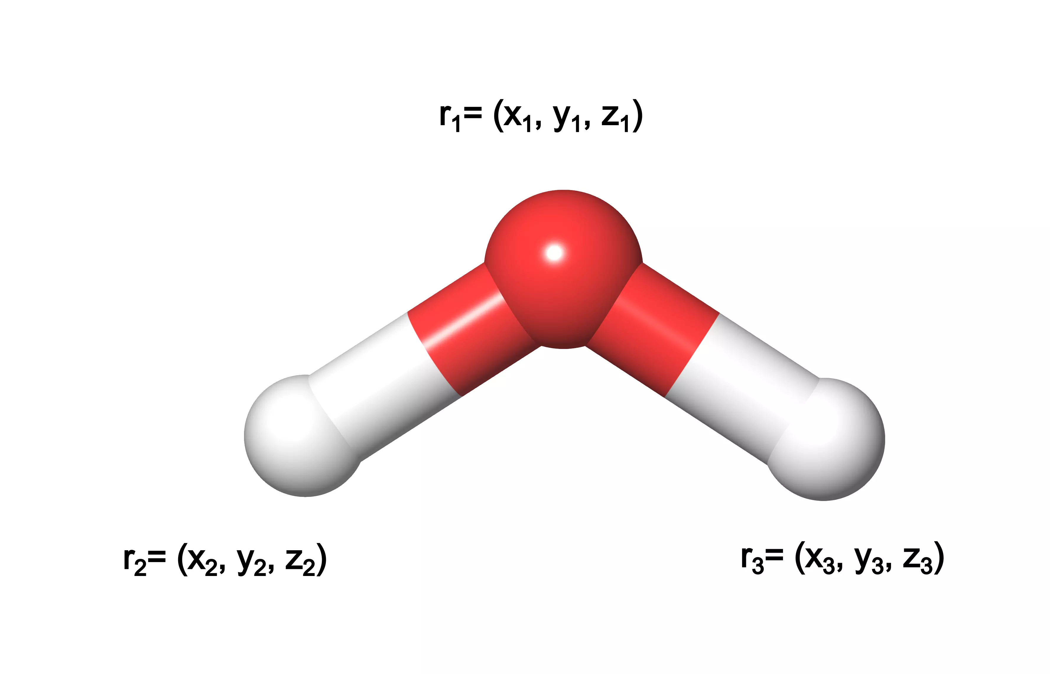
First of all, we need to consider that a molecule is composed of various atoms. At a certain time $t$, a given molecular geometry ($R$) composed of $N$ atoms can be expressed as a function of the $N$ atomic positions ($r_N$).
$$ R = (r_1, r_2, …, r_N) $$
Starting from here, successive configurations of the system are obtained by integrating Newton’s laws of motion ($F=ma$) for each atom.
Now we have two things to keep in mind.
1. The acceleration $a$ is the second derivative of the position $r$ with respect to time $t$.
Therefore, for each atom we can write:
$$ F_i = m_i \frac{\partial^2r_i}{\partial t^2} $$
where $F_i$ represents the force acting on the $i$-th atom.
2. The force is also equal to the opposite of the derivative of the potential energy $V$.
$$ F_i = -\frac{\partial V}{\partial r_i} $$
The analytical solution to the equations of motion is not obtainable for a system composed of more than two atoms. Therefore, to integrate the above equations we use a numerical approach named finite difference method.
The main idea behind this class of methods is that the integration can be divided into many small finite time steps $\delta t$. The time step needs to be small enough to correctly describe the process of interest. Since molecular motions are in the range of $10^{-14}$ seconds, a good $\delta t$ to describe them is typically in the order of femtoseconds ($10^{-15}s$). We will discuss this point in more detail later in this article.
At each step, all of the $N$ equations are simultaneously solved and the forces acting on each atom ($F_1,\dots,F_N$) at time $t$ are determined. From the force, we are then able to determine the acceleration.
$$ a_i = \frac{F_i}{m_i} = -\frac{1}{m_i} \frac{\partial V}{\partial r_i} $$
Finally, given the molecular position, velocity, and acceleration at time $t$, we are able to predict the position and velocity at the following time step ($t+\delta t$). This procedure is applied for many steps and the result is a trajectory that specifies how the positions and velocities of a particle vary with time.
The trajectory is not continuous but is just a series of configurations at different steps.
MD algorithm summary
- Initial conditions: Provide an initial configuration of the system consisting of the positions $r_i$, and velocities $v_i$ of the atoms at time $t$. Compute the potential energy $V$ arising from the interactions.
- Compute forces: The forces acting on each atom are retrieved from $V$. This is the most time-consuming step since the forces arise from interatomic interactions and depend on a broad variety of parameters.
$$ F_i =- \frac{\partial V}{\partial r_i} $$
- Find new configuration: The positions of atoms in the successive time step $t+\delta t$ are obtained by solving Newton’s equation of motion.
$$ a_i = \frac{F_i}{m_i} $$
- Iteration: We can update the initial configuration with the new one, and repeat the process for as many steps as needed.
The Verlet algorithm
From what we saw until now, it is clear that to retrieve the trajectory of a molecule one has to be able to integrate the equations of motion. However, we did not specify how this is achieved in practice yet.
To understand the mechanisms behind this procedure we first need to underline a concept that is central to nearly all the algorithms we use to obtain molecular motion. The majority of these techniques are assumed to be valid because the position, as well as the dynamical properties of a molecule at time $t+\delta t$, can be approximated through a Taylor expansion at time $t$.
$$ r(t+\delta t) = r(t) + \delta t v(t) + \frac{1}{2} \delta t^2 a(t) + \frac{1}{6} \delta t^3 b(t) + \dots $$ $$ v(t+\delta t) = v(t) + \delta t a(t) + \frac{1}{2} \delta t^2 b(t) + \dots \ $$ $$ a(t+\delta t) = a(t) + \delta t b(t) + \dots $$
where $v$ is the velocity, $a$ the acceleration, $b$ is the third derivative of the position with respect to time, and so on. This approximation gets better when the $\delta t$ is smaller.
As already stated, there are many algorithms to integrate Newton’s equation, providing a simulation of the motion of a molecule. The most widely used is a numerical method named the Verlet algorithm.
The latter uses the current positions $r(t)$ and accelerations $a(t)$, and the positions from the previous step $r(t - \delta t$) to retrieve the positions in the following step $r(t+\delta t$). The algorithm originates by simply writing the equations for the past and future positions:
$$ \mathbf{r}(t+\delta t) = \mathbf{r}(t) + \delta t \mathbf{v}(t) + \frac{1}{2} \delta t^2 \mathbf{a}(t) + \dots $$ $$ \mathbf{r}(t-\delta t) = \mathbf{r}(t) - \delta t \mathbf{v}(t) + \frac{1}{2} \delta t^2 \mathbf{a}(t) + \dots $$
and adding these two terms we have that:
$$ r(t + \delta t) = 2r(t) - r(t- \delta t) + \delta t^2 a(t) $$
which is the basic Verlet algorithm equation.
According to this principle, if we want to know the position of an atom in the future $r(t + \delta t)$ we need the position in the present $r(t)$ and in the past $r(t- \delta t)$ plus the present acceleration $a(t)$.
The Verlet algorithm mainly has two disadvantages:
- The equation does not incorporate velocities $v(t)$ explicitly and they need to be retrieved through additional calculations. Velocities are not needed to delineate the trajectory of a molecule, however, they are sometimes necessary to calculate some physical properties of the system (i.e., kinetic energy). The most basic way to estimate velocity is by using the mean value theorem. We compute it as $v = \Delta r / \Delta T$.
$$ v(t) = \frac{\big(r(t+ \delta t) - r(t - \delta t)\big)}{2\delta t} $$ $$ v(t + \delta t) =\frac{\big(r(t+ \delta t) - r(t)\big)}{2\delta t} $$
The main drawback of this method is that it generally leads to large errors.
- The basic Verlet algorithm requires the position from the previous step so it is not a self-starting algorithm. As a result, at $t=0$ the previous position $r(t-\delta t)$ needs to be identified by other means.
To overcome the deficiencies of the basic Verlet algorithm several variations have been developed. Here we provide a brief overview of two of the most important ones.
Velocity Verlet
The first one we are going to highlight is the velocity Verlet method, one of the most widely used in MD simulation. It derives from the position and the velocity Taylor expansions:
$$ r(t + \delta t) = r(t) + \delta t v(t) + \frac{1}{2} \delta t^2 a(t) $$ $$ v(t+ \delta t) = v(t) + \frac{1}{2}\delta t\big[a(t) + a(t + \delta t)\big] $$
The general idea is that we can the current position $r(t)$, velocity $v(t)$, and acceleration $a(t)$ to compute the motion of the molecule.
The procedure is articulated in three steps:
- Use the current position, velocity, and acceleration to obtain the position at the following time step $r(t + \delta t)$
- Once we updated the configuration of the system we can derive the resulting acceleration $a(t + \delta t)$ from the new forces acting on the atoms
- Finally, we can use $a(t + \delta t)$ to calculate the future velocity $v(t + \delta t)$ through the above equation.
Leapfrog algorithm
Another common alternative is the Leap frog method, which is based on the current position, and the velocity at time $t+\frac{1}{2}t$.
$$ v\left(t+ \frac{1}{2}\delta t\right) = v\left(t- \frac{1}{2}\delta t\right) +\delta ta(t) $$ $$ r(t + \delta t) = r(t) + \delta t v \left(t + \frac{1}{2}\delta t \right) $$
The main difference with the previous method is that we have a non-synchronous update of the coordinates and the velocities.
Initially we compute the velocities at time $t+\frac{1}{2}t$, and we use this information to compute the positions at the following time step $t+ \delta t$.
Then, the velocities “leap” again over the positions, and are retrieved at time step $t + \frac{3}{2}$, allowing us to find the positions at time step $t + 2\delta t$.
We reiterate the process for several time steps resulting in the trajectory of the molecule. Velocities and positions are mimicking two frogs jumping over each other, thus the name “leapfrog”.
Putting this into practice? The integrator, time step and constraints are all .mdp settings: integrator, dt, constraints. My complete GROMACS protein-in-water guide shows how to set them for a real run, from PDB file to analysed trajectory, with every MDP file and script included. Get the guide →
Changing integrator during an MD simulation
An MD experiment is composed of different steps during which we perform many simulations within different ensembles.
It is important to notice that it is not possible to switch integrator between Velocity Verlet and Leap Frog during the course of a simulation.
The reason for that lies in the fact that the velocities stored at each time step are different between the two integrators.
| Integrator | coordinates (r) and velocities (v) stored at each time step |
|---|---|
| Velocity Verlet | $[r_{t=0}, v_{t=0}], [r_{t=1}, v_{t=1}], [r_{t=2}, v_{t=2}],[r_{t=3}, v_{t=3}]$ |
| Leap Frog | $[r_{t=0}, v_{t=0,5}], [r_{t=1}, v_{t=1,5}], [r_{t=2}, v_{t=2,5}],[r_{t=3}, v_{t=3,5}]$ |
As you can see, while the coordinates stored at each time step are equal between the two integrators, the same is not valid for the velocities.
This will cause a discontinuity in the simulation, and will basically correspond to assigning new initial velocities to our system. In other words, any previous equilibration step will be made useless.
Selection of the time step and constraints
In Molecular Dynamics the motion is discretized into small finite time steps. The simulated time $T$ in an MD simulation is the product of the timesteps $\delta t$ and the number of timesteps $N_t$ calculated:
$$ T = N_t \delta t $$
In order to accurately describe molecular motion in molecular dynamics simulations, it is important to select an appropriate time step. Specifically, the time step must be small enough to capture the fastest motions within a molecule.
In biological systems, the fastest motions are represented by the oscillations of the hydrogen atom bound to a heavy atom (e.g., carbon). The period of bond oscillation of a $C-H$ bond is around $10 fs$. Hence, if MD should describe these motions the size of the integration time step should be in the order of ∼$fs$.
The time step to employ depends on the required numerical accuracy and also the integrating algorithm. The default choice is to employ a 1fs-long time step as it avoids severe energy leaks providing a reasonable accurate trajectory.
However, if we are not interested in sampling the fastest bond oscillations, it is possible to constraint them and employs larger time steps.
This procedure is similar to a coarse-graining of the system, and it acts as a low-pass filter for the oscillation motions. Constraining the length of covalent H atoms to their average bond length is a common practice in MD, and it allows for using a timestep as large as 2fs.
To constraint the bond lengths in a simulation we need to modify the equations of motion. To this aim, many algorithms have been developed. The most common ones are:
- SETTLE: it is mainly used to constraint water molecules. A fundamental task since water generally represents the majority of the simulation box.
- SHAKE: an iterative algorithm that resets all bonds to the constrained values. It also works for large molecules and can constraint bond angles.
- LINCS (LINear Constraint Solver): it is faster than SHAKE but is not able to constraint bond angles.
I will not go into the mathematical details of these algorithms. You can find more information in the official GROMACS documentation.