How to run a Molecular Dynamics simulation using GROMACS
GROMACS basic functions and commands
During your journey in Computational Chemistry, you will most likely come across different software used for molecular simulation. One of the most widely used is GROMACS, a free and open source software used to perform Molecular Dynamics (MD) simulations and to analyze the resulting trajectories.
If you are new to this world it can be frightening to go through the documentation and try to figure out how this program works. We have all been there.
Luckily for you, on this website, we have a detailed guide explaining to you how to perform simulation using GROMACS. Here I will give you a brief overview of the software as well as a general introduction to its basic commands.
However, before going through the tutorials I highly recommend you to check out my articles on Molecular Dynamics (MD) so that you can get a general idea of the technique, as well as the different steps involved in a simulation. Also, I will consider that you are quite comfortable with the concepts of:
What is GROMACS?
GROMACS is a versatile, high-performance molecular dynamics simulation package that can be used to study the behavior of molecules and biomolecules in various environments. It is particularly well-suited for simulating biomolecular systems, such as proteins, nucleic acids, and lipids, and has been widely used in a variety of fields, including chemistry, biology, and materials science.
One of the key features of GROMACS is its ability to perform highly efficient simulations using advanced algorithms and techniques making it possible to simulate large systems with millions of atoms, and to do so with high precision and accuracy.
GROMACS allows users to easily set up and run simulations, analyze the results, and also modify and optimize their simulations as needed. This makes it an ideal tool for researchers and scientists who are looking to study complex biomolecular systems and gain a better understanding of their behavior and interactions at the molecular level.
In addition to its powerful simulation capabilities, GROMACS also offers a wide range of advanced features and tools, such as support for free energy calculations and the ability to perform enhanced sampling methods. These features make it possible to study a wide range of phenomena and to tackle challenging research problems such as ligand binding or protein-protein interactions.
If you are interested in this software and you have no idea how to get started you are in the right place. Here is a guide on how to install GROMACS if you haven’t done that already.
Let’s begin.
Workflow
The general idea of GROMACS is not different from any other way of performing an MD simulation.
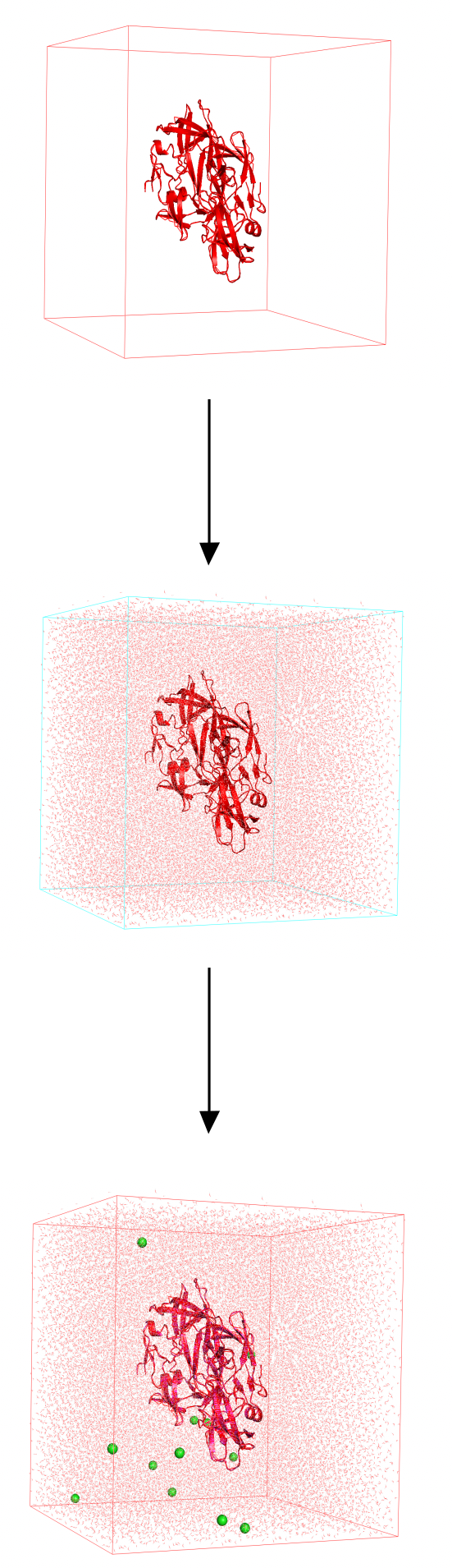
The first thing that we need to do is to prepare our system for the simulation. The system preparation phase is composed by three steps.
- Create a simulation box
- Solvate the system (e.g. using water)
- Neutralize the overall system using counterions ($Na^+$, $Cl^-$)
Once our system is ready we can proceed with the simulation phase.
- Energy minimization
- NVT equilibration
- NPT equilibration
- Production run
For each of these steps, we have specific commands to use and they require specific file formats.
Below you can find a list of the most common commands needed to carry out a simple MD simulation. The list is of course not exhaustive as the number of things you can do with GROMACS is immense.
Want the complete, hands-on version? This page walks through the workflow command by command. My GROMACS protein-in-water guide expands it into a full step-by-step project, from PDB file to analysed trajectory, with every MDP file, topology and script ready to run. Get the guide →
Commands
Let’s start with the basics.
Generally speaking, a GROMACS command can be seen as composed of four components:
|
|
gmxtells the computer we want to use GROMACS and is the starting point for each GROMACS command.- The
modulespecifies the operation we want to compute - Within each action, we have different flags (
-flag) that we can use - After the flag, we need to give GROMACS an
option, which can be a value or a file with some specific extension
gmx_mpi instead of the standard gmx.For each module you have different available flags and file formats you need to provide to the software. You can always refer to the official documentation to check for all the possible options within a command.
In addition you can get the available options for each module by typing;
|
|
As you may notice, the syntax for GROMACS is quite easy. Let’s see how it works in practice.
System preparation
In the initial phase of our experiment, we need to set up our system. The workflow involves four commands:
- pdb2gmx
- editconf
- solvate
- genion
System preparation workflow
Let’s consider the commands involved in more detail.
gmx pdb2gmx
It is very likely that you have the starting structure for your minimization as a PDB file (More info on PDB files here). However, you will need to convert it into files that can be used by GROMACS.
The first command we are going to need is pdb2gmx, which is needed to generate three files.
topol.top: The topology file will contain force field parameters information for each atom in the structure. This includes bonding as well as non bonding parameters.posre.itp: A position restraint file that will be useful in the equilibration step of our simulation.protein.gro: An output structure in the gro format. The result is a coordinate file that will have x, y, and z coordinates for each atom of the structure in it, much like a simple PDB file.
This will be the starting point for our GROMACS simulation. If you are interested, you can find more info on these GROMACS file formats here.
The command is the following:
|
|
- Call the program with
gmx - Select the
pdb2gmxmodule - Call the
-fflag and provide the starting PDB structureprotein.pdb - Select the
-oflag and decide how you want to name the output file - The
-waterflag allows us to select the water model we want to use
pdb2gmx will give you an error if you have an incomplete structure that lacks some residues. Make sure to reconstruct the missing residues via homology modeling.Once you launched the command you will be asked to choose the Force Field you desire.
|
|
gmx editconf
The editconf command defines the size and shape of the box for our simulation.
|
|
- Call the program with
gmx - Select the
editconfcommand - Select the
-fflag and provide the starting structure (protein.gro) - Call the
-oflag and decide how you want to name the output file (protein_box.gro) - The
-cplaces our system in the center of the box - Choose the
-dflag and place our system at the selected distance from the box (at least 1.0 nm in our case) - Decide the shape of the simulation box with the
-btflag
gmx solvate
The name says it all. We use this command to solvate the box.
|
|
- Call the program with
gmx - Select the
solvatecommand - Select the
-cpflag and provide the starting structure for the solute (protein_box.gro) - Specify the solvent with the
-csflag. The default solvent is Simple Point Charge (spc) water - Call the
-oflag and decide how you want to name the output file (protein_solv.gro) - Finally, we use the
-pflag and provide the previously generated topology file
gmx genion
In the final step of the system preparation, we use the genion command to replace solvent molecules with ions. By adding ions we are able to neutralize the system.
|
|
- Call the program with
gmx - Select the
genioncommand - Select the
-sflag and provide the .tpr file for the ions (ions.tpr) - Call the
-oflag and decide how you want to name the output file (system.gro) - Use the
-pflag and provide the topology file (topol.top) - Choose the
-pnameflag to decide the name of the positive ions name - The
-nnameflag is used to decide the name of the negative charge ions - The
-neutralflag tells GROMACS to neutralize the net charge of the system
grompp command which is discussed below.Once you launched the command you will be asked to choose the atoms you want to replace with ions. Here, you will have to select the solvent as you don’t want to substitute protein atoms right?
Simulation
At this stage, we have our system ready to be simulated.
As already mentioned, the simulation phase involves multiple steps. A typical MD protocol consists of different simulations carried out within different ensembles.
All of them are simply based on two commands, regardless of the type of simulation we want to run:
- grompp: we use it to generate an input file in the tpr format
- mdrun: we run the simulation using the previously generated tpr file
GROMACS Simulation workflow
Overall, the workflow to perform a simulation is extremely intuitive. Let’s analyze the commands more in-depth.
gmx grompp
The grompp command is necessary to assemble:
- A coordinate file (
system.gro) - A topology file (
topol.top) - An mdp file containing the parameters for our simulation (
simulation.mdp)
As a result, we get a .tpr file with coordinates, topology, and parameters for minimization. Now we can use this file to run the simulation.
Simple right?
|
|
- Call the program with
gmx - Select the
gromppcommand - Select the
-fflag and provide the mdp file with the parameters for the run (simulation.mdp) - The
-cflag is used to provide the coordinates of atoms - The
-rflag is needed if we are using position restraints. Mostly during the equilibration steps of your simulation. - In some cases we may want to continue our simulation starting from a previous one. To this aim, we can use the
-tflag coupled with a previously generated cpt file. - Use the
-pflag and provide the topology file (topol.top) - Call the
-oflag and decide how you want to name the output file (simulation.tpr)
gmx mdrun
Finally, we are ready to launch the simulation with the mdrun command.
|
|
- Call the program with
gmx - Select the
mdruncommand - The
-vmakes the command verbose. It is useful to make clearer what the program is actually doing while running. - The
-deffnmoption is followed by the prefix of the tpr file we are using. This will generate files having the same prefix.
(simulation.tpr $\Rightarrow$ -deffnm simulation)
After completion you will generally get five files:
simulation.logcontaining information about the runsimulation.growith the final structure of the systemsimulation.edrwith energies that GROMACS collects during the simulationsimulation.xtca “light” weight trajectory with the coordinates of our system in low precisionsimulation.trrwith the higher precision trajectory of positions, velocities, and forces during the simulation
You can use these files to perform a variety of different analysis.
Check out the article where I show you how you can extract thermodynamic properties from an edr file.
Simulation Tutorials
Now that you know the basics of this software you can check the tutorials on how to run an MD simulation using GROMACS. Two of them are available for now. I suggest that you run them in the specified order.