GROMACS Tutorial: Molecular Dynamics simulation of a protein in water environment

Background for molecular simulation

In this tutorial, we are going to see from a practical point of view how to simulate a protein in a water environment using GROMACS.

Most of the commands and functions needed to carry out a successful Molecular Dynamics (MD) simulation were already discussed in other articles.

I strongly suggest you read the article where I introduced GROMACS article before going through this tutorial so that you can have:

1. A general idea of how GROMACS works.
2. A proper understanding of the commands involved in a basic GROMACS simulation

Throughout the course of the tutorial, I will still redirect you to a more detailed description of the commands when needed. Feel free to click on those links to have a more clear explanation of each step.

I am going to assume that you have a general idea of the different concepts involved in a Molecular Dynamics (MD) simulation. I link you to a category of articles dedicated to the subject where you can find some useful concepts that you should be familiar with for a proper understanding of this tutorial.

A problematic aspect of GROMACS is that sometimes the simulation will run regardless of whether you have a clear idea about what you are doing or not. When you will start running your own simulations you will discover that it will be fundamental to know what is going on behind the scenes so that you can properly set your own parameters, and debug eventual errors.

I will also take for granted that you are more or less familiar with the Linux command line.

Having clarified that, we are ready for the tutorial.

System preparation

An MD simulation requires different steps. I will not go into the detail of each step, you can find more information about the different steps required to carry out an MD simulation here.

In the first step of the simulation, we need to select the protein and proceed to prepare the system for the experiment.

Protein Selection and initial setup

For this tutorial, we are going to consider a small structure that does not require extensive simulation times. The chicken villin subdomain will do just fine (PDB ID: 1YRF).

You can download the structure here, and then visualize it with your favorite visualization software. You can check this PyMOL introduction if you want more detail on how to visualize a molecular structure

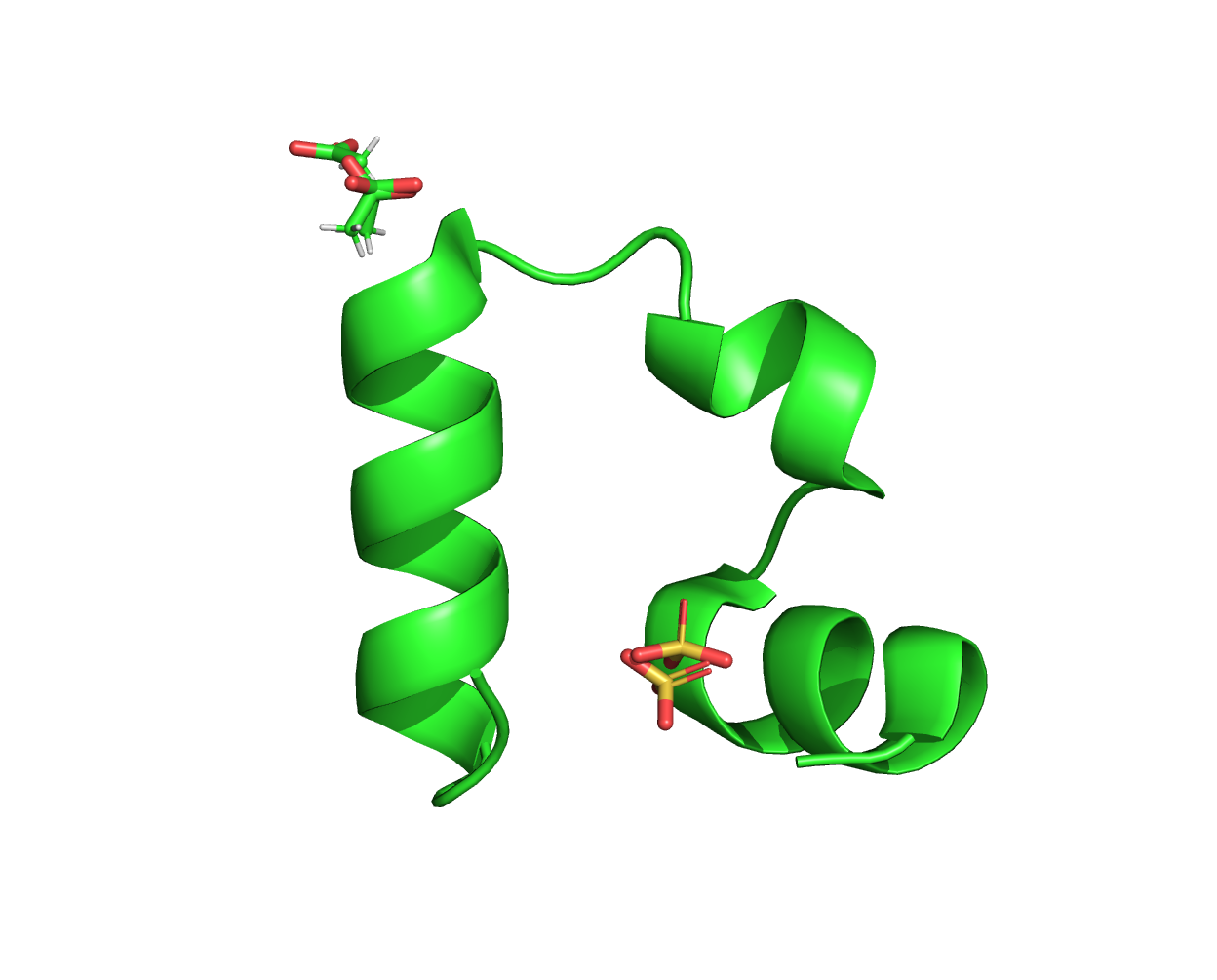
First of all, we need to delete the water and the ligands from the pdb file. You can do it with your favorite text editor but the most common way to do it is to use the grep command like this:

1

grep -v HETATM 1yrf.pdb > 1yrf_clean.pdb

Now we need to create a topology for our protein. To this aim, we are going to use the pdb2gmx command as follows:

1

gmx pdb2gmx -f 1yrf_clean.pdb -o 1yrf.gro -water tip3p -ignh

GROMACS will ask us to select a Force Field (FF).

 1
 2
 3
 4
 5
 6
 7
 8
 9
10
11
12
13
14
15
16

Select the Force Field:
 1: AMBER03 protein, nucleic AMBER94 (Duan et al., J. Comp. Chem. 24, 1999-2012, 2003)
 2: AMBER94 force field (Cornell et al., JACS 117, 5179-5197, 1995)
 3: AMBER96 protein, nucleic AMBER94 (Kollman et al., Acc. Chem. Res. 29, 461-469, 1996)
 4: AMBER99 protein, nucleic AMBER94 (Wang et al., J. Comp. Chem. 21, 1049-1074, 2000)
 5: AMBER99SB protein, nucleic AMBER94 (Hornak et al., Proteins 65, 712-725, 2006)
 6: AMBER99SB-ILDN protein, nucleic AMBER94 (Lindorff-Larsen et al., Proteins 78, 1950-58, 2010)
 7: AMBERGS force field (Garcia & Sanbonmatsu, PNAS 99, 2782-2787, 2002)
 8: CHARMM27 all-atom force field (CHARM22 plus CMAP for proteins)
 9: GROMOS96 43a1 force field
10: GROMOS96 43a2 force field (improved alkane dihedrals)
11: GROMOS96 45a3 force field (Schuler JCC 2001 22 1205)
12: GROMOS96 53a5 force field (JCC 2004 vol 25 pag 1656)
13: GROMOS96 53a6 force field (JCC 2004 vol 25 pag 1656)
14: GROMOS96 54a7 force field (Eur. Biophys. J. (2011), 40,, 843-856, DOI: 10.1007/s00249-011-0700-9)
15: OPLS-AA/L all-atom force field (2001 aminoacid dihedrals)

For this tutorial, we are going to Select “6” (AMBER99SB-ILDN)

We will generate three files from this run:

• A structure file (1yrf.gro)
• A topology file (topol.top)
• Position restraints (posre.itp)

You can find more info on these file formats here

Define a box

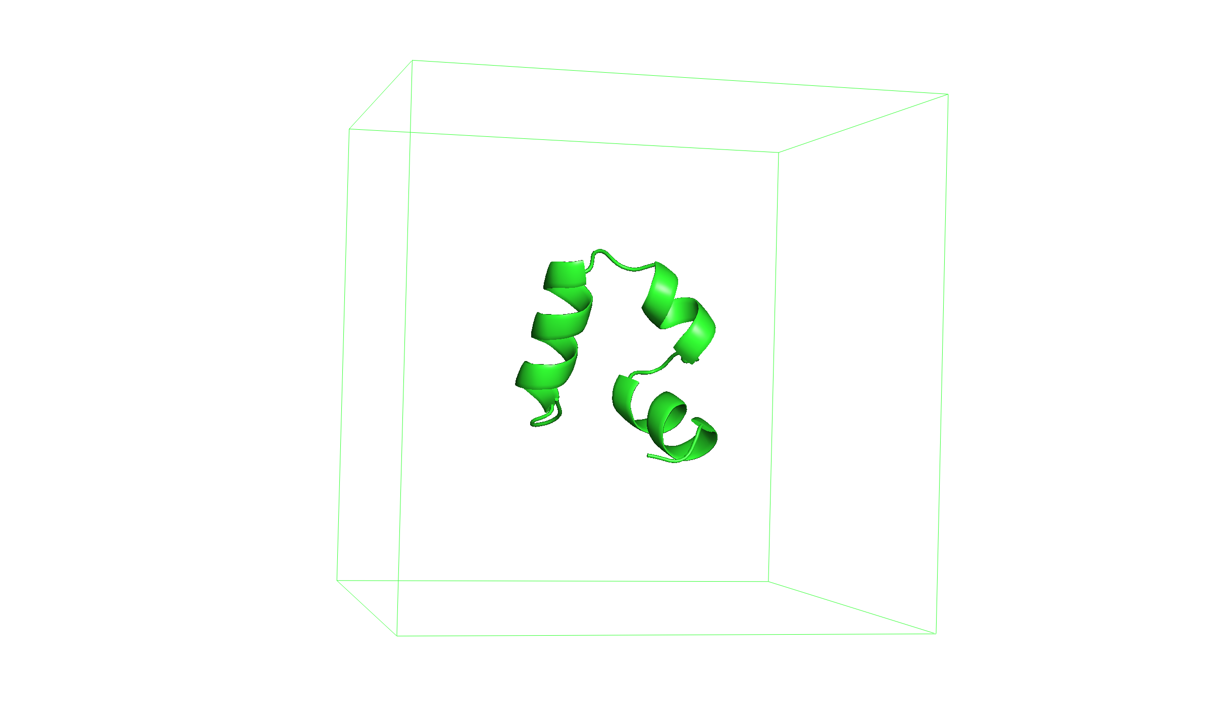
At this stage, we need to create a virtual simulation box for our protein. You can do it with the editconf module.

1

gmx_mpi editconf -f 1yrf.gro -o 1yrf_box.gro -c -d 1.0 -bt cubic

We will need the protein to be at least 1.0 nm from the edge of the box to make sure that we don’t have problems when implementing Periodic Boundary Conditions (PBC).

You can load the resulting structure (1yrf_box.gro) with Pymol and use the command show cell to show the box containing the protein.

Solvate the system

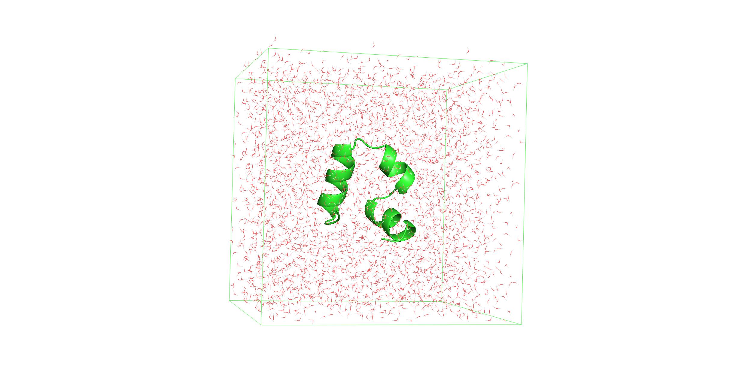
Now we need to add solvent to the system through the solvate module. As already stated, we are going to use water as a solvent.

Type the following command:

1

gmx solvate -cp 1yrf_box.gro -cs spc216.gro -o 1yrf_solv.gro -p topol.top

You will generate a new gro file named 1yrf_solv.gro. If you open the file with Pymol you should see something that looks like Figure.

Neutralize

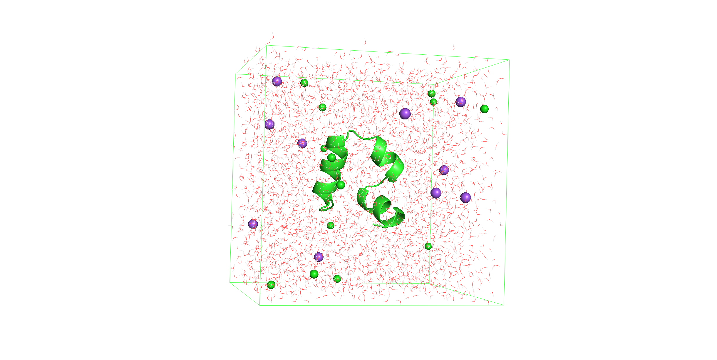
The last step of our system preparation phase consists of neutralizing the system by adding ions. This is accomplished via the genion module.

To use this module we first need a file containing the tpr file (ions.tpr) that is going to be used as input.

To generate it we need to use the grompp module. To use the grompp module we need an mdp parameter file (ions.mdp).

This may seem a little bit confusing if you are not familiar with GROMACS. This diagram may help to clarify the situation.

We need an ions.mdp file to use the grompp module. You can download it from here.

You can assemble the ions.tpr file with this command:

1

gmx grompp -f ions.mdp -c 1yrf_solv.gro -p topol.top -o ions.tpr

Now we can use this file as input for the genion module.

1

gmx_mpi genion -s ions.tpr -o 1yrf_ions.gro -p topol.top -pname NA -nname CL -neutral -conc 0.15

The genion module neutralizes the system by replacing some molecules in our system with ions.

GROMACS will ask us to select the molecules we want to replace with ions. We want to select the solvent (water molecules in our case) so that they will make place for the ions..

 1
 2
 3
 4
 5
 6
 7
 8
 9
10
11
12
13
14
15
16
17

Will try to add 11 NA ions and 13 CL ions.
Select a continuous group of solvent molecules
Group     0 (         System) has 11595 elements
Group     1 (        Protein) has   582 elements
Group     2 (      Protein-H) has   289 elements
Group     3 (        C-alpha) has    35 elements
Group     4 (       Backbone) has   105 elements
Group     5 (      MainChain) has   141 elements
Group     6 (   MainChain+Cb) has   174 elements
Group     7 (    MainChain+H) has   177 elements
Group     8 (      SideChain) has   405 elements
Group     9 (    SideChain-H) has   148 elements
Group    10 (    Prot-Masses) has   582 elements
Group    11 (    non-Protein) has 11013 elements
Group    12 (          Water) has 11013 elements
Group    13 (            SOL) has 11013 elements
Group    14 (      non-Water) has   582 elements

Select the solvent “13 SOL”.

The resulting gro file (1yrf_ions.gro) will be used for the simulation.

Simulation

The second phase of this tutorial consists of actually simulating the system we prepared.

The simulation procedure involves multiple steps.

1. Energy minimization
2. NVT equilibration
3. NPT equilibration
4. Production run

They are all based on two modules:

1. grompp
2. mdrun

The general idea is similar to what we saw for the genion module.

We use the grompp module to assemble a tpr input file. The difference is that we run the input file with the mdrun command.

We will need an mdp parameter file for each run to define the simulation settings. The mdp templates are discussed in more detail here.

Energy minimization

This procedure aims to minimize the potential energy of the system by adjusting the atomic coordinates. It will stabilize the overall structure and avoid steric clashes.

Download the mdp parameter file (minim.mdp) from here.

Use the grompp module to generate a tpr file for the energy minimization (em.tpr).

1

gmx grompp -f minim.mdp -c 1yrf_ions.gro -p topol.top -o em.tpr

Now you can run the simulation with the mdrun command.

1

gmx mdrun -v -deffnm em

Depending on your computational resources this process may take from a few seconds to minutes.

The mdrun module generates four files:

• em.gro: containing the final structure
• em.log: information about the run
• em.trr: with the trajectory of the system
• em.edr: an energy file useful for the analysis of the simulation

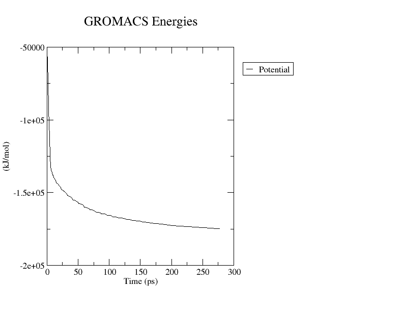
We can use this last file to observe how the energy gets minimized along the simulation with the gmx energy module. This module will generate a file in the xvg format that we can use to generate a plot.

1

gmx energy -f em.edr -o potential.xvg

At the prompt, type:

1

10 0

to select Potential energy.

You can plot the resulting xvg file (potential.xvg) using Grace. Find a more detailed description of the gmx energy module and the xmgrace tool here.

1

xmgrace potential.xvg

This should be the result.

You can also download the initial structure (1yrf_ions.gro) and compare it to the new one (em.gro) by loading both of them in Pymol.

NVT equilibration

The energy minimization ensured that we have a reasonable starting structure, in terms of geometry and solvent orientation. Before proceeding with the actual simulation we need to perform an equilibration procedure. This is needed to equilibrate the ions and the solvent around the protein.

We will divide it in two phases.

The first one will be carried within the NVT ensemble. This means that we are going to implement a thermostat, and we will equilibrate the system at constant temperature.

We are going to run a 100 ps simulation using the V-rescale thermostat.

Find the nvt.mdp file needed to run the grompp module here.

1

gmx grompp -f nvt.mdp -c em.gro -r em.gro -p topol.top -o nvt.tpr

Now you can run the simulation with this command

1

gmx mdrun -v -deffnm nvt

Starting from now, the simulations will be more computationally intensive. Depending on the machine you are using this process could take some time.

Once the simulation is over we can use the gmx energy to extract properties from the run.

In NVT equilibration the temperature of the system should reach a plateau at the value we specified in the mdp file. Let’s see how long it takes for the temperature to reach a stable value.

1

printf "16 0" | gmx energy -f nvt.edr -o nvt_temperature.xvg

Plot the xvg file.

1

xmgrace nvt_temperature.xvg

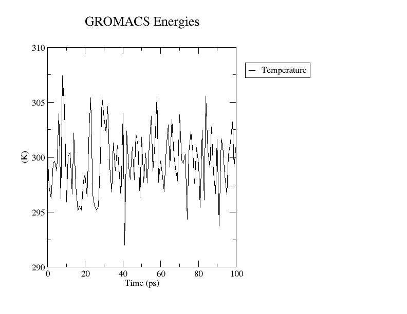
As you can see the temperature is quite stable around the selected value (300K). In general, if the temperature has not yet stabilized, additional time will be required.

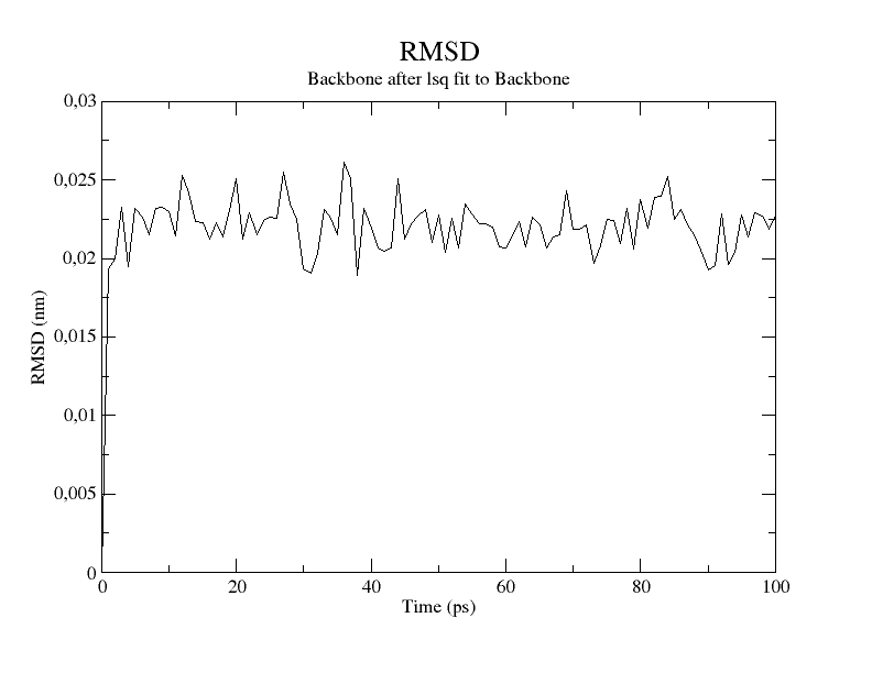
To check that the system is properly equilibrated we can check the RMSD value via the gmx rms module.

1

printf "4 4" | gmx rms -f nvt.trr -s nvt.tpr -o nvt_rmsd.xvg

This will output an xvg file (nvt_rmsd.xvg) with the backbone to backbone RMSD for the protein. Let’s plot it.

1

xmgrace nvt_rmsd.xvg

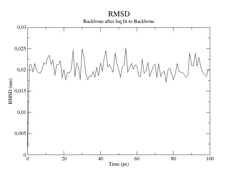
The RMSD quickly converges to a stable value signaling that the system has equilibrated at the desired temperature. We can move to the next phase.

NPT equilibration

The second equilibration will be carried out within the NPT ensemble. In this case, we are going to bring the system at constant pressure through a virtual barostat. We will run a 100 ps simulation using the Parrinello-Rahman barostat.

Download the npt.mdp parameter file here.

Assemble the tpr file with the grompp command, and then launch the simulation with mdrun.

1

gmx grompp -f npt.mdp -c nvt.gro -r nvt.gro -t nvt.cpt -p topol.top -o npt.tpr

1

gmx mdrun -v -deffnm npt

We can monitor the progression of the pressure with the gmx energy module as previously shown.

1
2

printf "18 0" | gmx_mpi energy -f npt.edr -o npt_pressure.xvg;
xmgrace npt_pressure.xvg

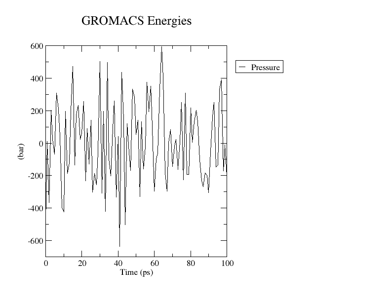
You can see that the protein widely fluctuates around the pressure value we selected in the mdp file (1 bar). Don’t worry, large pressure fluctuations are completely normal for nanoscale simulations of aqueous solutions.

Once again, we can check the RMSD value to control that the system has properly equilibrated at constant pressure.

1
2

printf "4 4" | gmx rms -f npt.trr -s npt.tpr -o npt_rmsd.xvg
xmgrace npt_rmsd.xvg

The RMSD values are very stable over time, indicating that the system is well-equilibrated at the desired pressure.

Production run

Now that our system is finally equilibrated at the desired temperature and pressure we are ready for the real simulation. This is the so-called production run.

During this phase, we are going to release the position restraints on the heavy atoms of the protein. We will observe how the system evolves over time, and depending on our goal we will collect relevant data.

The production run will still be carried out within the NPT ensemble using the V-rescale thermostat and the Parrinello-Rahman barostat.

For the purpose of demonstration, we are just going to perform a 1 ns simulation. Keep in mind that in a real experiment you will need to run hundreds of ns to extract useful information from your system.

Find the md.mdp file here.

1

gmx grompp -f md.mdp -c npt.gro -t npt.cpt -p topol.top -o md.tpr

1

gmx mdrun -v -deffnm md

The production run will be a little bit longer than the previous one. If you want to run it in background use:

1

nohup gmx mdrun -v -deffnm md &

This will append the output in a temporary file named nohup.out

You can check the progress of the simulation with the following command:

1

tail -f nohup.out

When the simulation is over you will still find the relevant informations in the usual files (md.edr, md.log, md.xtc)

Congratulations! you have now successfully conducted your MD simulations. This ends the tutorial.

However, GROMACS comes with a lot of tools to analyze the trajectory of a protein. We already saw some practical examples of the gmx energy and the gmx rms modules. Feel free to use these commands to analyze the results of this run.

Yuo shouldn’t stop here. Analyzing your system is like putting together a puzzle, the more pieces you have the clearer the picture gets.

For this reason, you can find other articles dedicated to a series of analysis you may be interested in performing for your research:

• Analyze the hydrogen bonds with the gmx hbond module
• Compute the RMSF with the gmx rmsf module
• Estimate the Solvent Accessible Surface Area (SASA) via the gmx sasa module
• Cluster your trajectory to find the most representative structure of the simulation

Pro Tip

Here you can find a list of the commands we used to carry out the simulation. It is always useful to have them in a file so that you can simply copy and launch them from the terminal.

Just remember to change the name of the initial pdb file.

In the end, you can find links to the .mdp file templates.

System preparation

1
2
3
4
5

gmx pdb2gmx -f (protein.pdb) -o protein.gro -water tip3p  
gmx editconf -f protein.gro -o protein_box.gro -c -d 1.0 -bt cubic
gmx solvate -cp protein_box.gro -cs spc216.gro -o protein_solv.gro -p topol.top 
gmx grompp -f ions.mdp -c protein_solv.gro -p topol.top -o ions.tpr 
gmx genion -s ions.tpr -o system.gro -p topol.top -pname NA -nname CL -neutral -conc 0.15

Simulation

1
2
3
4
5
6
7
8

gmx grompp -f minim.mdp -c system.gro -p topol.top -o em.tpr
gmx mdrun -v -deffnm em 
gmx grompp -f nvt.mdp -c em.gro -r em.gro -p topol.top -o nvt.tpr
gmx mdrun -deffnm nvt 
gmx grompp -f npt.mdp -c nvt.gro -r nvt.gro -t nvt.cpt -p topol.top -o npt.tpr
gmx mdrun -deffnm npt 
gmx grompp -f md.mdp -c npt.gro -t npt.cpt -p topol.top -o md.tpr
gmx mdrun -deffnm md

mdp files

ions.mdp

em.mdp

nvt.mdp

npt.mdp

md.mdp