How to study Hydrogen bonds using GROMACS

GROMACS comes with a broad set of tools to perform analysis on our Molecular Dynamics (MD) simulation.

One particular structural feature one may be interested in investigating is the Hydrogen bond interactions in our system. As a matter of fact, the analysis of hydrogen bonds plays an important role in the field of molecular simulation.

For this reason, GROMACS allows us to study hydrogen bonds via a specific module named gmx hbond.

This tutorial will walk you through the theory and process of using hydrogen bond analysis to investigate your system of interest.

Hydrogen bonds in Molecular Dynamics simulations

Let’s start from the beginning.

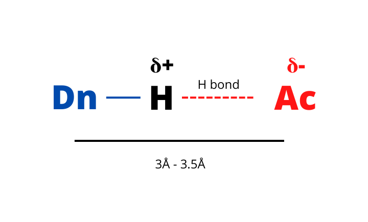
The formation of a hydrogen bond involves three participants:

1. Donor (Dn): a highly electronegative atom (F, O, N) covalently linked to an H atom.
2. Acceptor (Ac): another highly electronegative atom (F, O, N) not covalently linked to an H atom.
3. Hydrogen (H): a hydrogen atom shared between the donor and the acceptor.

Hydrogen bonds are a special class of interactions of particular interest in the field of MD simulation.

Despite being regarded as a “weak interaction” hydrogen bonds play a fundamental role in the context of biological systems.

On the one side, these interactions are important for structural reasons, since they stabilize the secondary structure of proteins. On the other side, they are also of great importance in stabilizing protein-ligand complexes.

As a result, the characterization of the H-bond interactions is particularly relevant in the MD simulation of protein-ligand complexes, and therefore in the field of computational drug discovery.

It is generally useful to study the number and/or duration of H-bond interactions between a ligand and a protein along the course of the simulation.

Different tools are nowadays available. In this article, we will only focus on the gmx hbond module provided by GROMACS.

The gmx hbond module

The gmx hbond module determines the hydrogen bonds entirely based on geometry. More specifically, the H-bond interactions among two groups are based on two cutoffs:

• The Ac–Dn–H angle between the three atoms involved in the hydrogen bond.
• The distance between the two heavy atoms involved in the interaction (Ac–Dn).

When the angle and the distance are below a given cutoff the interaction is considered a hydrogen bond.

Considering what was previously mentioned it is clear that GROMACS considers by default electronegative atoms covalently linked to H atoms (OH, NH) as donors while the N and O atoms are regarded as acceptors.

How to compute the hydrogen bonds between two groups

The gmx hbond module allows us to count the number of H-bonds between two groups (e.g., between two residues or between a protein and a ligand) at each frame of our simulation.

This can be useful when you want to determine how important is the formation of a certain H-bond interaction in your simulation. For instance, you can retrieve information on the relevance of a certain interaction between a ligand and a protein by considering how often it forms in your simulation.

The workflow is quite intuitive. You provide two groups via an ndx file, and GROMACS computes the number of interactions depending on the cutoff and writes them in an output file in the xvg format.

The first step of this analysis is to create an index file via the gmx make_ndx with the groups you need. This is optional but in most cases, you will want to define special groups other than the default groups provided by GROMACS.

Then you can use the gmx hbond module as follows:

1

gmx hbond -f md.xtc -s md.tpr -n index.ndx -num hbnum.xvg

You will be asked to select the two groups you want to analyze. The result will be an output file in the xvg format that you can plot as you wish. Here I showed how to plot an xvg file using Grace or Python.

For instance:

1

xmgrace hbnum.xvg

The graph will be something resembling the figure below.

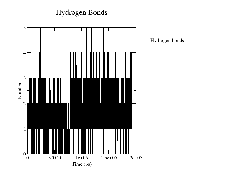
Number of Hydrogen bonds as a function of time (ps) graphed with Grace

Now you can see the number of hydrogen bonds between the two specified groups at each frame of the simulation. In our example, the number of H bonds between the two selected groups mostly range between 1 and 3.

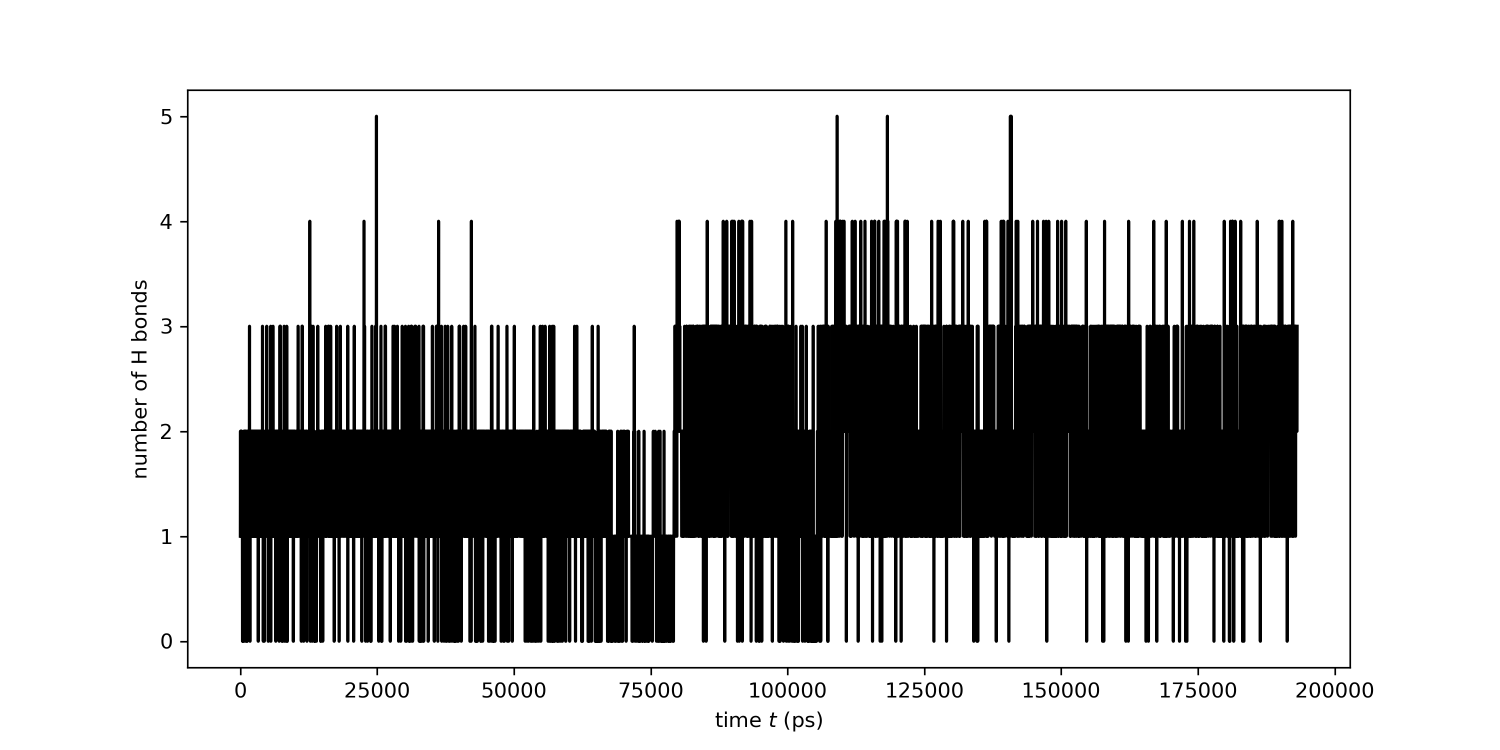
You can also generate a plot using Python (Numpy and Matplotlib).

 1
 2
 3
 4
 5
 6
 7
 8
 9
10
11
12
13
14
15

import matplotlib.pyplot as plt
import numpy as np

t,hbond,pairs = np.loadtxt("hbnum.xvg", comments=["@", "#"], unpack=True)

fig = plt.figure(figsize=(10,5))
ax = fig.add_subplot(111)


ax.plot(t,hbond, color="black", linestyle="-")
ax.set_xlabel("time $t$ (ps)")
ax.set_ylabel("number of H bonds")

plt.savefig("hbnum.png", format="png", dpi=300)
plt.show()

List of atoms involved in Hydrogen bonds

The gmx hbond module can also be used to create an index file containing the atoms involved in hydrogen bond interactions. The idea behind this analysis is very similar to the previous one. You will still need to provide the two groups you want to analyze via an index file but in this case, we will get another ndx file as output.

Also, the command is very similar to the one previously shown:

1

gmx hbond -f md.xtc -s md.tpr -n index.ndx -hbn hbond.ndx

After you selected the two groups GROMACS will give you the hbond.ndx file as output. You can open it with your favorite text editor or you can look at it with the gmx make_ndx module:

1

gmx make_ndx -f md.gro -n hbond.ndx

Let’s say you considered two groups (A and B) the groups contained in the index file should be something like this:

1
2
3
4
5
6
7

  0 A             :  4382 atoms
  1 donors_hydrogens_A:   892 atoms
  2 acceptors_A   :   706 atoms
  3 B         : 256190 atoms
  4 donors_hydrogens_B: 211732 atoms
  5 acceptors_B: 57861 atoms
  6 hbonds_A-B: 32523 atoms

In other words, you will get groups containing donors and acceptor atoms for both A and B. Additionally, you will have listed all the atoms involved in hydrogen interactions between the two groups (hbonds_A-B).