GROMACS Tutorial: How to simulate a protein in membrane environment
Part 2
Membrane proteins are a particular class of proteins that are able to interact with biological membranes.
In recent years, membrane proteins have been raising in popularity, and a large number of studies simulating these systems are now available.
This is now possible because of two reasons:
- The increasing computational capacity at our disposal allows us to deal with more complex systems
- The increasing number of available membrane protein structures (e.g., in the Protein Data Bank (PDB)).
The simulation of a membrane protein can be more challenging than a normal simulation of a protein in a water environment.
For this reason, this is intended as an intermediate tutorial. I am going to assume that you are familiar with GROMACS and with the different concepts involved in a Molecular Dynamics (MD) simulation.
If you are not, please first check out the beginner level GROMACS tutorial where I showed you how to simulate a protein in water. When needed, I will still redirect you to other relevant articles on this website.
New to GROMACS? This membrane tutorial is intermediate and assumes the basics. If you want those fundamentals first, my GROMACS protein-in-water guide takes you from a PDB file to a fully analysed trajectory, with every MDP file and script included. Get the guide →
A protein membrane system is composed of tens of thousands of atoms (if not hundreds). For this reason, they require an extensive amount of computational power.
This tutorial makes no exception.
Make sure to run the simulations involved in this tutorial on a specialized workstation. Alternatively, you can modify the parameters for the run and perform shorter simulations to reduce the computational time.
File Preparation
The system we will consider is a small transmembrane peptide (PDB ID: 2MG1) embedded in a cholesterol membrane.
You can check the previous part of this tutorial to check how we built the protein membrane system we are going to simulate.
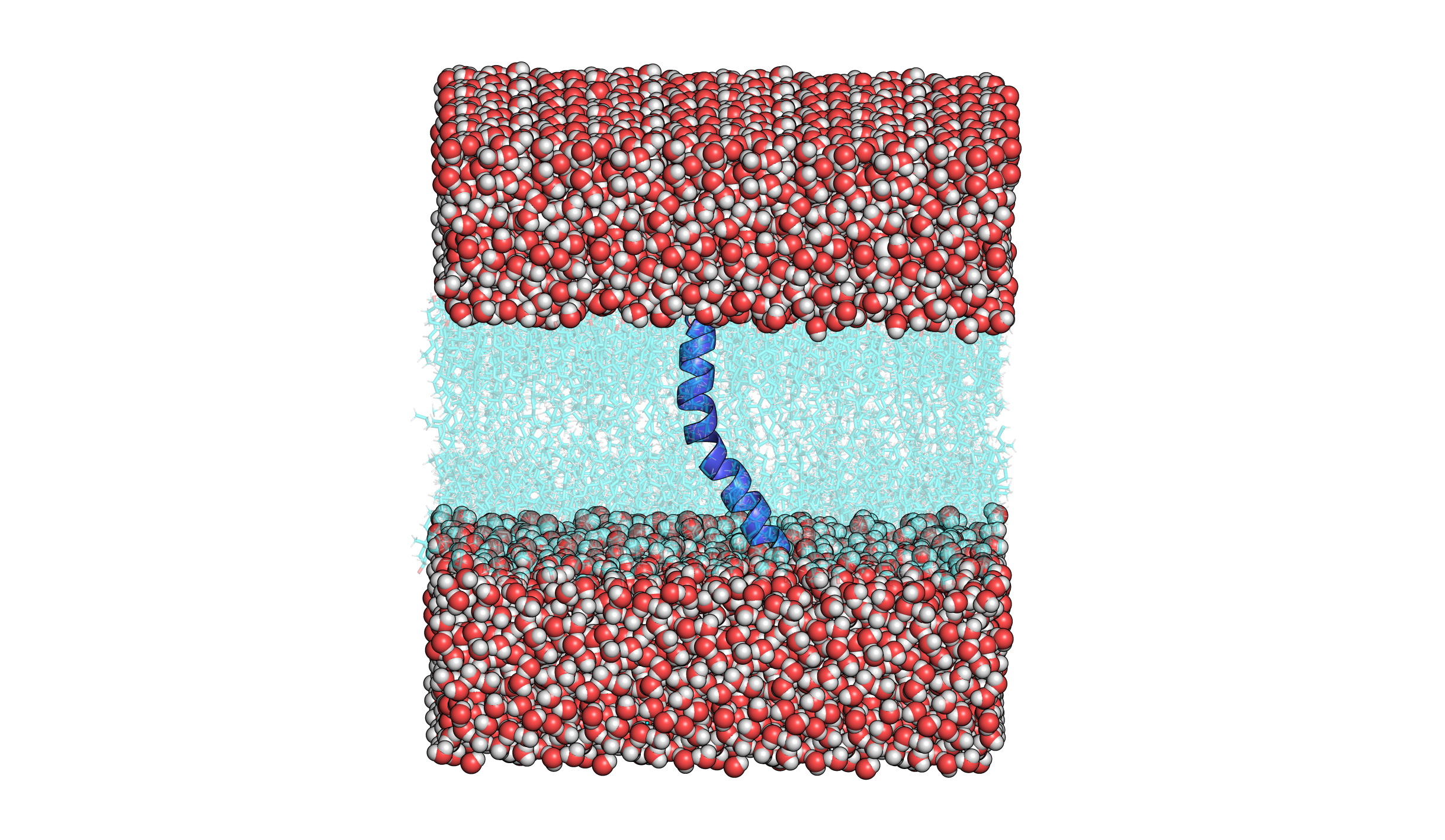
Transmembrane peptide (Blue) embedded in cholesterol membrane, and water molecules as solvent (Red).
Otherwise, you can download the file required for the simulation here.
First of all, we need to unpack the tgz file we created through CHARMM-GUI in the previous part of this tutorial.
|
|
Now enter the resulting directory:
|
|
Inside it, you wil find three files:
- The topology for the system (
topol.top) - The structure of the system in the gro format (
step5_input.gro) - A directory (
toppar) containing the position restraints (itp files) for the different types of species involved in the simulation.
You can find more info on these file formats here
At this stage, we will also need to create a special index via the gmx make_ndx module. This will be useful later on.
More specifically, we need to create an index file with two special groups. The first one contains the protein and the membrane, and the second one contains the solvent (water and ions).
|
|
Select the protein and the membrane
|
|
Then rename the new group as follows:
|
|
Also, create an index group for the solvent
|
|
Again let’s rename the group.
|
|
When you are done quit with q
Workflow
The simulation is going to be divided into different steps.
The general idea is similar to the one we discussed in the article where I showed the different steps required to set up an MD simulation. However, we will need a few adjustments.
When dealing with complex systems is generally advisable to be more careful with the equilibration procedure. A fast equilibration may result in the “explosion” of the system, and we may result in the creation of holes in the membrane.
Therefore, we will add a few additional equilibration steps to make sure the system is properly equilibrated.
The workflow will be this:
- Minimization: the usual potential energy minimization.
- Simulated annealing: here we are going to slowly bring the system to the desired temperature (1ns simulation).
- NVT: a simulation within the NVT ensemble (constant Temperature). We will perform three different 5ns NVT simulations slowly decreasing the restraints on the membrane while retaining the ones on the protein (1+1+1=3ns).
- NPT: a 10ns simulation within the NPT ensemble (constant pressure) with restraints on the protein.
- Production run: a simulation within the NPT ensemble and no restraints (50ns).
For each of this step we will need a different mdp file with the parameters for the run. Feel free to change the duration of each run depending on the computational resources you have.
For this relatively simple system, a more straightforward equilibration protocol might still be sufficient. However, I’ve opted to present a more cautious approach to familiarize you with various techniques that can be crucial for equilibrating more complex systems. This includes the gradual heating and the stepwise reduction of restraints.
Remember, the equilibration protocol we choose for our simulation is heavily dependent on the specific characteristics of the system. Each protocol should be tailored to suit your particular case.
All of the preliminary steps are just intended as equilibration steps. Therefore, only aim is to make sure that the system is able to equilibrate without exploding. I’ve chosen to share a protocol that should generally be effective across a wide range of systems, but feel free to adapt it to your preferences.
For simpler systems, such as the one featured in this tutorial, a more straightforward equilibration approach might suffice. For more complicated systems you may need to be more careful and release the restraints more slowly or perform longer equilibrations.
A common alternative is to use the mdp files generated by the CHARMM-GUI membrane builder, forming a six step equilibration protocol.
The parameters, thermostat, and barostat that you decide to use get more relevant in the production run since that one is used to extract data from your simulation.
I found myself more comfortable with generating a different directory for each step to keep the terminal clear, as we will generate a large number of files. Feel free to run everything in a single directory but it will get quite messy.
We are going to create seven different directories.
|
|
Energy minimization
The first step will be energy minimization. Enter the minimization directory.
|
|
Download the mdp file for energy minization. Then assemble the tpr file for the energy minimization via the gmx grompp module.
|
|
Then run the calculation with the gmx mdrun module.
|
|
We can observe the variation in the potential energy using the gmx energy module (in the linked article I also show you how to plot the results of this analysis).
|
|
At the prompt select the Potential energy.
This will give us an xvg output file that we can plot using your favorite tool. Grace could be right what you need when you only want a quick plot of GROMACS xvg output.
|
|
Simulated Annealing
One of the negative occurrences that can happen in a protein simulation in a membrane environment is the creation of holes in the lipidic membrane. In other words, the system may explode especially if we are not careful enough with our equilibration procedure.
The annealing procedure is needed to gradually bring the system to the desired temperature to avoid the previous situation.
In our example, we are going to bring the system to 300K in 1ns.
Go the the annealing directory.
|
|
Download the mdp file for the annealing. Now we can assemble the tpr file and launch the simulation.
|
|
The simulation time for the steps involved in this protocol could be extremely long. In such cases, it is always useful to launch the mdrun command using nohup.
|
|
This will append the output to a file named nohup.out instead of the standard output file. You can check the progress of the simulation with the following command:
|
|
When the simulation is over you will still find the usual output files (anneal.edr, anneal.xtc, anneal.log, …)
We can look at the temperature gradually increasing in time.
|
|
It is also interesting to notice the change in volume occurring during the simulation.
|
|
NVT equilibration
Now we will run three NVT simulations slowly decreasing the restraints on the lipidic membrane. All of them are going to use the Berendsen thermostat.
This is not the most sophisticated thermostat algorithm at our disposal. However, it can be extremely useful in the equilibration step where we just want to bring our system to the desired temperature no matter what. It is generally advisable to select other thermostats for production runs.
Go to the nvt_1 directory.
|
|
Download the mdp file and then assemble the tpr file for the first simulation.
|
|
|
|
Then we only need to repeat this procedure two times.
First, we are going to perform a second NVT simulation with looser restraints on the membrane.
Go to the nvt_2 directory (Download the mdp file for nvt_2)
|
|
Run the simulation
|
|
Finally, we will completely release the restraint on the membrane and run the last step of our NVT simulation. (mdp file for nvt_3)
|
|
|
|
NPT equilibration
From now on the steps will be quite similar to the ones that were explained in other protocols.
First of all, we need to perform an NPT equilibration. During this phase, we will bring the system to the desired pressure through a virtual barostat. We will use the Parrinello-Rahman barostat and perform a 10ns equilibration at T = 310K.
Download the mdp file for the NPT run.
|
|
|
|
Now we have our system equilibrated and ready to be simulated.
Production run
In the last step of this experiment, we are going to completely release the restraints on the protein and perform a 50ns unbiased simulation.
We are going to use a more sophisticated thermostat (Nosè-Hoover) coupled to the Parrinello Rahman barostat to maintain constant Temperature = 310K and Pressure = 1 bar.
Download the mdp file for the production run.
|
|
|
|
Now you can proceed to analyze the results of the analysis as you wish.
List of commands and mdp files
Here is the list of commands as well as the mdp files we used for the tutorial.
Minimization and annealing
|
|
Equilibration
|
|
Production
|
|