GROMACS Tutorial: Coarse-Grained simulation of a protein membrane system
In the previous tutorial, we introduced the Martini force field and its application to simulating proteins in aqueous environments.
Now, let’s take a step further and explore the exceptional capacity of coarse-grained (CG) simulations. These methods are uniquely suited for modeling extensive systems, making them the perfect choice for simulating protein membrane systems.
Throughout this tutorial, I’ll provide step-by-step guidance on simulating proteins in membrane environments, using the Martini force field. It’s worth noting that many concepts discussed here were previously covered in the first article, and the simulation protocol will have many similarities.
Should any questions arise, don’t hesitate to reference the earlier article for clarification. However, I highly recommend reviewing the first part before continuing further for a comprehensive understanding.
Simulation Workflow
Before starting, as always, here is the protocol we will use in this tutorial.
It closely aligns with what we covered in the previous tutorial and shares many similarities with a standard MD procedure. However, the crucial difference lies in the conversion of the structure from atomistic to coarse-grained and the subsequent system preparation. In this context, we go beyond the incorporation of water and ions; we also construct the membrane complete with its diverse components.
Download and Prepare the Protein Structure
To kickstart our membrane protein simulation, our first step involves obtaining an atomistic structure from the Protein Data Bank.
In this tutorial, we’ll use the adenosine A2a receptor, a prominent member of the G-protein coupled receptor family known for its crucial role in signal transduction (PDB ID: 3PWH). However, if you have a different protein in mind that piques your interest, feel free to proceed with it. Just keep in mind that you may need to adjust the commands and mdp files accordingly.
As a crucial first point, we need to make sure that the protein is properly aligned along the z axis. This alignment is crucial for the subsequent embedding process into the membrane, as we will see in the upcoming steps.
For this reason, the first thing we need to do is to download the structure properly aligned. We can do this using the OPM web server.
You can access the server at this link. There, select Search for PDB entry, input the PDB ID of the protein (in this case, 3PWH), then click Search and Submit query. You’ll be directed to a page where you’ll need to wait a few minutes. Eventually, you’ll be able to download the oriented protein structure, which you can save as 3pwh_opm.pdb.
As always, it’s essential to clean the protein structure from any non-protein elements. This can be accomplished using the grep command:
|
|
This will ensure that we’re working with a clean and aligned representation of the protein.
Convert the structure to CG with Martinize
Next, we’ll utilize the powerful Martinize Python script to convert our atomistic membrane protein structure into a coarse-grained (CG) representation and generate the corresponding topology file. For detailed instructions on how to install Martinize, please refer to the previous article.
|
|
- The command begins with
martinize2, which is the executable for themartinize2tool. - The
-fflag is used to specify the input atomistic structure file in PDB format. In this case, it is3pwh_clean.pdb. - Provide the secondary structure via the
-dsspflag (More info in previous article). - The
-xflag is used to specify the output file name for the converted CG structure. Here, the name3pwh_cg.pdbis chosen for the coarse-grained structure file. - Select the
-oflag and name the topology (topol.top). The topology file will contain all the information about the system - Select the Martini 3 force field with
-ff martini3001 - The
-scfixflag applies side-chain corrections. - The
-cysflag is set toauto, which allows the program to automatically detect disulfide bonds in the protein and create appropriate constraints. - The
-p backboneoption defines position restraints on the backbone. - The
-elasticflag activates the elastic network model. Elastic networks are used to introduce harmonic constraints between pairs of atoms within a certain cutoff distance, simulating the connectivity and flexibility of the protein. - The
-ef,-el, and-euflags control the parameters for the elastic network.-ef 700.0sets the force constant for the elastic network springs to 500 • kJ/mol/nm$^2$,-el 0.5defines the lower cutoff for interactions, and-eu 0.9specifies the upper cutoff. These parameters determine the strength and range of the harmonic constraints in the elastic network.
While we’re using the default settings for elastic networks and cutoff values in this demonstration, I highly recommend conducting experiments with different parameters and evaluating the fluctuations, including Root Mean Square Deviation (RMSD) and Root Mean Square Fluctuations (RMSF).
Compare these values to those obtained from a parallel simulation at the all-atom (AA) level. This comparative analysis will provide insights into how closely your CG system mirrors its AA counterpart. The closer the fluctuations align, the more accurate your CG model represents the AA structure.
This will generate three files:
- the CG structure (
3pwh_cg.pdb) - The corresponding topology (
topol.top) - The CG parameters file for the protein (
molecule_0.itp)
Embedding the Protein in the Membrane using Insane
To create the system we can take advantage of the insane.py script. You can obtain the script from here.
To embed in a model membrane having 50% cholesterol and 50% POPC you can use this command:
|
|
Let’s break down the options and parameters of this command:
-
-f 3qak_cg.pdb: Specifies the input CG structure file (in PDB format) of the protein. -
-o 3qak_memb_cg.gro: Sets the name of the output file for the solvated system in GROMACS GRO format. -
-p topol.top: Specifies the topology file containing system connectivity and force field parameters. -
-l POPC:50 -l CHOL:50: Defines the membrane composition of the lower leaflet (50% cholesterol, 50% POPC). -
-l POPC:50 -l CHOL:50: Defines the membrane composition of the upper leaflet (50% cholesterol, 50% POPC). -
-x 14 -y 14 -z 14: Defines the system size in the x, y, and z dimensions, respectively, in nanometers. These values determine the size of the water box. -
-sol W:100: Indicates the type and number of solvent molecules to add. In this case, it adds 100 water molecules (W) to solvate the system. -
-salt 0.15: Specifies the salt concentration in moles per liter (M). In this case, it adds salt ions to achieve a concentration of 0.15 M. -
-center: Centers the solvated system within the simulation box.
Recall the importance of aligning the protein along the z axis, as mentioned earlier. Well, note that we can use this script only because we preciously aligned the protein on the z-axis. Failing to do so could result in the protein being arranged in an incorrect orientation, potentially leading to undesired outcomes.
Before progressing further, always take the time to visually inspect the system, ensuring that the structure aligns logically. In our case, the system closely resembles the typical embedding of a G-protein coupled receptor (GPCR) within a membrane.
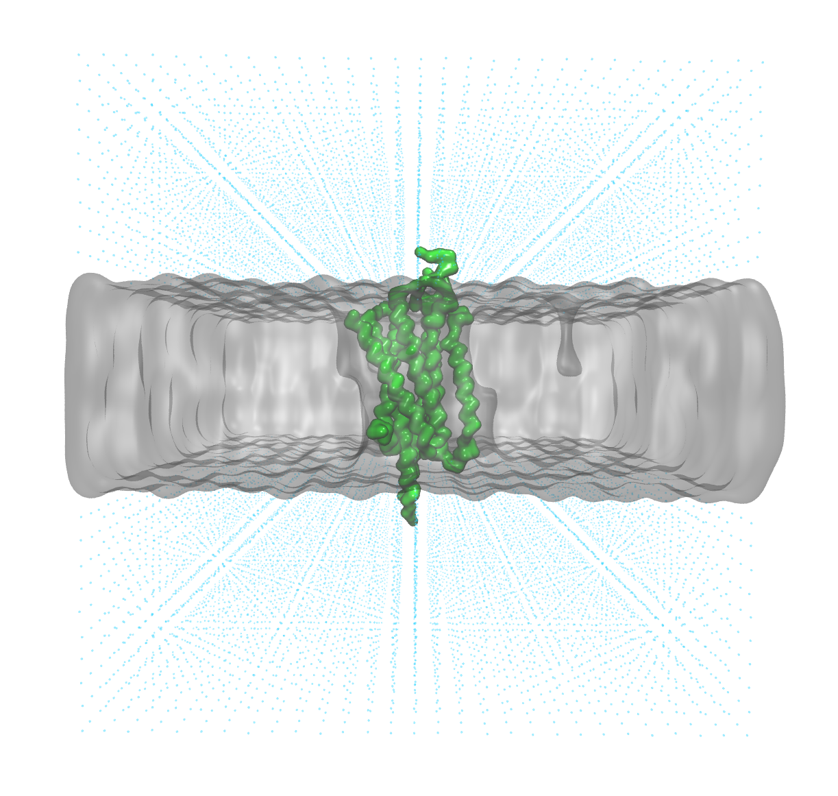
The protein (green) has the correct orientation with respect to the membrane (grey surface)
Martini itp files
The final step before running the simulation is to adjust the topology file including all the required itp files for each of the components for the Martini force field.
The itp files for the Martini 3 force field can be downloaded here. Unpack this file using the following command:
|
|
Inside you will find a directory containing four files:
- General parameters:
martini_itp/martini_v3.0.0.itp - Phospholipids:
martini_itp/martini_v3.0.0_phospholipids_v1.itp - Water:
martini_v3.0.0_solvents_v1.itp - Ions:
martini_v3.0.0_ions_v1.itp
You can now move the file that was previously generated for the protein (molecule_0.itp) to the martini_itp directory.
|
|
Finally, integrate all of these files into the topology file (topol.top). These should be the first lines in your topol.top file:
|
|
Also in the [ molecules ] section of our topology file, we need to change Protein with molecule_0.
This is how the file should look like this in the end.
|
|
Simulation
With the structure downloaded, aligned along the z-axis, and embedded in the membrane, we can now proceed into the simulation phase.
This phase closely mirrors the protocol of a standard Molecular Dynamics (MD) simulation. The key steps include minimization, equilibration, and culminate in the production run.
Once you start the simulations, you will immediately notice a distinct advantage in performance with respect to a classical simulation. Using the CG technique you can easily simulate in the µs timescale, an objective that would pose significant challenges with atomistic resolution.
Minimization
Now, we will create a dedicated directory named minim to neatly organize and store the results of this step.
|
|
Next, you will need to download the mdp file for the minimization run and copy that into this directory.
Navigate into the newly created directory to initiate the minimization process with the following commands:
|
|
|
|
Equilibration protocol for CG simulations
CG systems are more stable so we need a rough equilibration. We are going to stick to 50 ns NPT simulation.
To begin, we need to create an index.ndx file to store the membrane and solvent groups separately. These groups will be treated independently by the thermostat and barostat during the equilibration process. Additionally, you can also take the chance to create a group of atoms including the backbone (a BB) for future calculations, such as computing the root-mean-square deviation (RMSD).
|
|
|
|
|
|
Now you can download the mdp file for the NPT run here.
|
|
Then run the simulation
|
|
Production run
Finally, we will run a 1 μs production run following the usual procedure. Note that this would take weeks to simulate at an atomistic level, while here the process is much faster and should probably finish in less than one day.
Create a directory and move into it.
|
|
Download the mdp file for the production run here, then you can use it to generate the md.tpr file.
|
|
Run the simulation in background:
|
|
Congratulations! You’ve successfully completed the simulation of your membrane protein.